One-Way ANOVA Statistical Guide: Mastering Analysis of Variance

Discover the essential techniques of One-way ANOVA Statistical Guide to discern and analyze group differences effectively, elevating the accuracy and depth of your dataset analysis.

---

Introduction

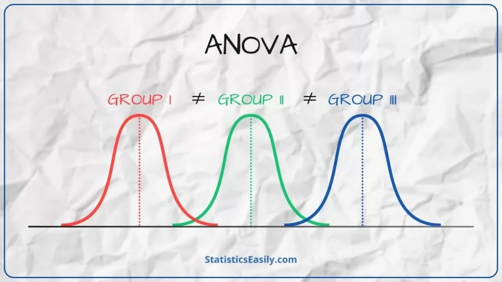
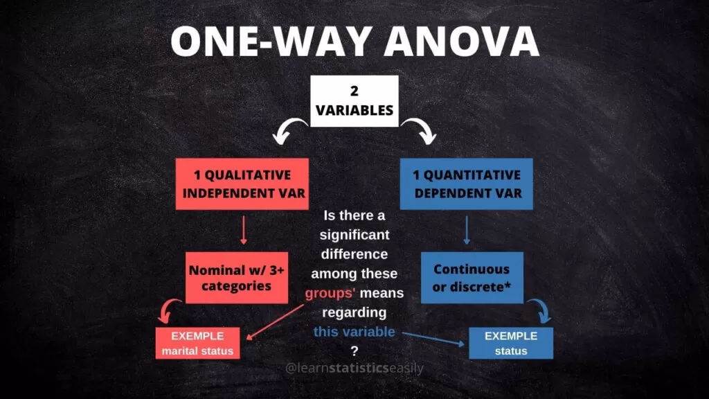
One-way ANOVA is a cornerstone statistical method for comparing the means across three or more independent groups. This test is pivotal in discerning whether the observed differences in sample means are statistically significant or could have occurred by chance. Essentially, One-way ANOVA examines the influence of a single categorical independent variable on a continuous dependent variable, providing insights into the variance within and between defined groups.

One-way ANOVA is paramount in research domains where comparing multiple groups is essential. It is extensively applied in fields such as psychology, education, medicine, and any scientific inquiry that requires the rigorous validation of experimental results. By deploying this analysis, researchers uphold the integrity of their conclusions, ensuring that they reflect the true nature of the data rather than the randomness of variability.

This guide is meticulously structured to facilitate a deep understanding of one-way ANOVA and its application. Beginning with a foundational theory, we investigate when and why this statistical test should be employed. The subsequent sections systematically explore the assumptions of One-way ANOVA, the step-by-step process of performing the analysis in SPSS, and the interpretation of results. Post-hoc analyses, reporting standards, and graphical representation techniques are elucidated to aid in comprehensive understanding. This educational journey is designed to impart the knowledge to master One-way ANOVA and apply it confidently in research endeavors.

---

Highlights

1. One-way ANOVA effectively compares means across three or more groups, revealing significant differences beyond chance.
2. Essential for integrity in scientific research, ANOVA underpins rigorous validation of experimental results across various fields.
3. ANOVA’s F-statistic, a key metric, objectively assesses between-group mean disparities, which is crucial for data accuracy.
4. Post-hoc tests in ANOVA pinpoint statistically significant differences, controlling for Type I errors in multiple comparisons.
5. When ANOVA’s assumptions are not met, alternatives like Welch’s ANOVA or non-parametric tests offer robust solutions.

---

Theoretical Foundation

The one-way ANOVA is a critical statistical tool used in hypothesis testing when comparing the means of three or more groups. In this context, hypothesis testing is a formal methodology for investigating our research questions, allowing us to make inferences about population parameters based on sample statistics. The role of ANOVA, or Analysis of Variance, here is to test for significant differences across group means, providing a single test statistic — the F-statistic — to assess the null hypothesis that no differences exist.

The null hypothesis for a one-way ANOVA (denoted as H0​) posits that all group means are equal, formally expressed as H0​:μ1​=μ2​=…=μk​, where μ represents the group mean, and k denotes the number of groups. Rejecting this hypothesis implies that at least one group mean is statistically different from the others, warranting further investigation into these disparities.

Understanding group mean differences is paramount in many scientific domains as it influences decision-making and policy formation. One-way ANOVA empowers researchers to discern whether observed variations in means are substantive and thus warrant further attention or are simply due to chance. Mastery of this method enables the exploration of data with precision and the extraction of meaningful insights, ensuring that research findings align with the pursuit of the true, the good, and the beautiful in scientific inquiry.

---

When to Use One-Way ANOVA?

One-way ANOVA is particularly valuable in study designs where the primary interest is comparing the means of three or more groups subject to different levels of a single treatment or condition. This includes randomized controlled trials and observational studies where the independent variable is categorical, and the dependent variable is measured continuously.

One-way ANOVA is appropriate when:

1. You have three or more independent groups subjected to distinct treatments.
2. The groups are mutually exclusive, meaning each subject belongs to one group only.
3. The aim is to determine if there is a significant difference in the means of the groups.

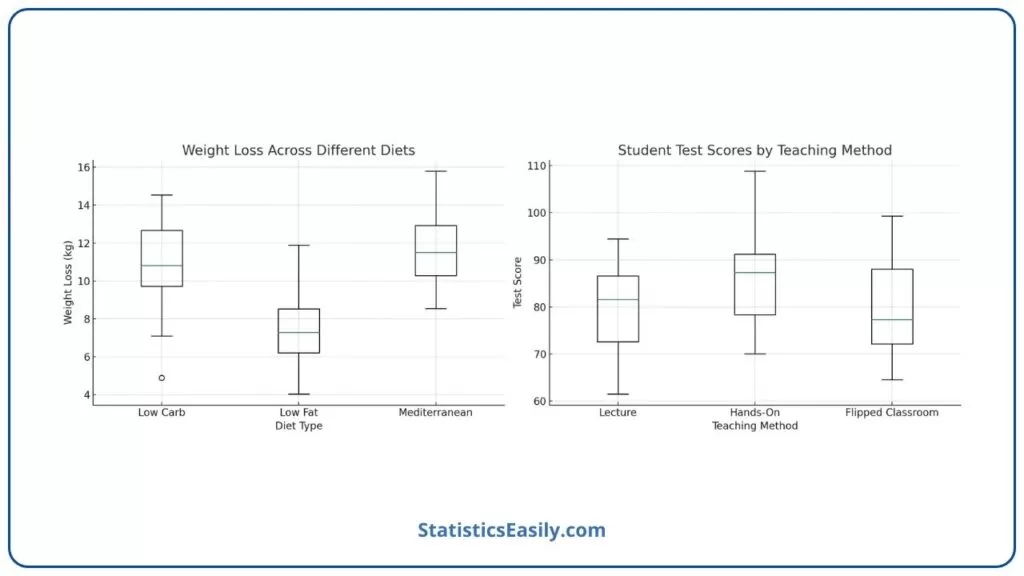
For example, a researcher investigating the effect of different diets on weight loss might assign subjects to a low-carb diet, a low-fat diet, or a Mediterranean diet. The one-way ANOVA would compare the mean weight loss between these three groups to ascertain if diet type has a significant effect. Another practical example is an educator comparing the test scores of students taught using different teaching methods. By assigning one group to a traditional lecture, another to a hands-on approach, and a third to a flipped classroom, the educator can use one-way ANOVA to evaluate which method leads to the highest academic performance.

---

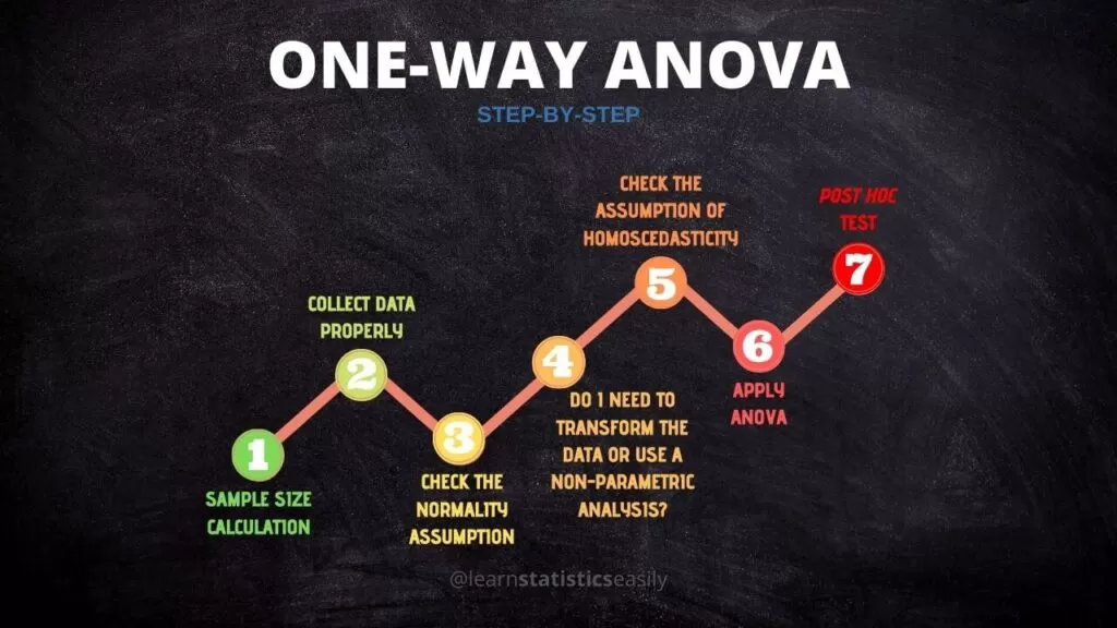
Statistical Assumptions of One-Way ANOVA

One-way ANOVA requires several vital assumptions to ensure the validity of its results. Firstly, the normality assumption stipulates that the group’s residuals should follow a normal distribution. Homogeneity of variances, also known as homoscedasticity, demands that the residual groups’ variance be approximately equal. Lastly, independence of observations asserts that the observations must be independent of each other, typically satisfied by a well-designed randomization process.

How do you test these assumptions using software?

Testing these assumptions involves a few steps:

1. Normality: can be assessed using Shapiro-Wilk’s test or visually through Q-Q plots.
2. Homogeneity of Variances: Levene’s test is commonly used to examine homoscedasticity.
3. Independence of observations: is usually assured during the study design phase. However, it can be checked by ensuring no patterns are present in a plot of the residuals.

How do you proceed when assumptions are not met?

When these assumptions are not met, the researcher has several options:

1. Data transformation or non-parametric tests like the Kruskal-Wallis test can be considered if normality is violated.
2. When homogeneity of variances is not present, adjustments to the ANOVA model, such as using Welch’s ANOVA, may be appropriate.
3. If the independence of observations is questioned, the study design may need to be revisited, or a different statistical method should be employed.

---

Step-by-Step Guide to One-Way ANOVA in R

Data Preparation and Input

Before conducting a one-way ANOVA, ensure your data is appropriately formatted. The dependent variable in one column should be continuous, and the independent variable in another should be categorical, indicating group membership. Confirm that your data meets the assumptions of ANOVA: normality, homogeneity of variances, and independence of observations.

Detailed Instructions on Running One-Way ANOVA in R

1. Enter Data: First, input your data into R. Create a data frame with one column for the dependent variable (a continuous variable) and another for the independent groups (a categorical variable). For example:

your_data <- data.frame(
  dependent_variable = c(...),  # Continuous data here
  independent_variable = factor(c(...))  # Group labels here
)

2. Load Required Packages: Install and load necessary packages. You need the stats package for a basic ANOVA, which comes pre-installed with R.

install.packages("stats")
library(stats)

3. Run the ANOVA Test: Use the aov() function from the stats package. Example:

result <- aov(dependent_variable ~ independent_variable, data = your_data)

4. View ANOVA Summary: Use the summary() function to view the ANOVA results, including the F-statistic, degrees of freedom, and p-values.

summary(result)

5. Post Hoc Tests (If Necessary): If your ANOVA result is significant (p-value < 0.05), you may want to conduct post hoc tests to determine which specific groups differ. Use TukeyHSD() for Tukey’s Honestly Significant Difference test.

if(summary(result)[[1]]$'Pr(>F)'[1] < 0.05) {
  posthoc_results <- TukeyHSD(result)
  print(posthoc_results)
}

6. Check Assumptions: Normality: Use the shapiro.test() on the residuals of the ANOVA model.

shapiro_test_result <- shapiro.test(residuals(result))
print(shapiro_test_result)

• Homogeneity of Variances: Use the bartlett.test() function.

bartlett_test_result <- bartlett.test(dependent_variable ~ independent_variable, data = your_data)
print(bartlett_test_result)

7. Calculate Effect Size: The effect size can be calculated as Eta Squared or Omega Squared. R has no built-in function for this, but you can calculate it manually or use additional packages. Example using Eta Squared:

eta_squared <- sum(result[[1]]$'Mean Sq')[1] / (sum(result[[1]]$'Mean Sq')[1] + sum(result[[1]]$'Mean Sq')[2])
print(eta_squared)

8. Reporting the Results: When reporting the results, include the F-statistic, p-value, degrees of freedom, and effect size. Discuss the results in the context of your research question. If significant, identify which groups differ (based on post hoc tests) and the magnitude of these differences (effect size).

Interpreting the Output from One-Way ANOVA in r

ANOVA Table: When you use `summary(result)` in R, it shows the ANOVA table. This table includes key figures like the F-statistic, p-value, and degrees of freedom.

• F-statistic: This number tells you how much the group means differ. It’s calculated by comparing the variance (difference from the average) between groups to the variance within groups. A higher F-statistic usually suggests a more significant difference between group means.
• Degrees of Freedom: These numbers relate to the number of groups and data points. They provide context for interpreting the F-statistic. There are two types: ‘between groups’ and ‘within groups’.
• P-value: The p-value helps you decide if your results are significant. If it’s below a certain threshold (often 0.05), it suggests that the differences in group means are unlikely to be due to chance. A low p-value means you can reject the null hypothesis (which states no differences between the groups).
• Effect Size: This measures the strength of the relationship between the groups. It’s not just about whether the groups are different (that’s what the p-value tells you) but how different they are. Use functions like `eta_squared()` or `omega_squared()` from R packages to calculate this. Effect size gives more insight into the practical significance of your results.

Significant F-statistic: If the F-statistic is high and corresponds to a low p-value, this indicates a significant difference between some group means. in this case, you should perform post hoc tests to see which specific groups differ from each other.

Non-Significant F-statistic: If the F-statistic is low or the p-value is high, this suggests that the differences between group means are not statistically significant. This might prompt a review of your study design or consideration of other statistical methods.

---

Post Hoc Analysis

After you find a significant result in One-Way ANOVA, it’s vital to conduct post hoc tests. These tests help identify which specific group means are different from each other, as the ANOVA test alone only indicates that there is a difference without specifying where it lies.

Key Post Hoc Tests:

Tukey’s Honestly Significant Difference (HSD): Best for all pairwise comparisons, especially when group sizes are equal. Use `TukeyHSD()` in R for this test.

Bonferroni Correction: Suitable for a small number of comparisons. It’s a conservative method that adjusts the significance level to control for Type I error. Apply this correction using `pairwise.t.test()` with the `p.adjust.method = “bonferroni”` parameter.

Scheffé’s Test: Ideal for complex comparisons, particularly when the number of groups is large. Implement with the `schefe.test()` function from appropriate R packages.

Games-Howell Test: Useful when the assumption of homogeneity of variances is violated. It’s a nonparametric test and can be applied using the `gamesHowellTest()` function from relevant R packages.

Choosing the Right Test: The choice of post hoc test is influenced by factors like the homogeneity of variances, group sizes, and the number of comparisons. If variances are unequal, consider using Games-Howell as it does not assume equal variances.

Conducting Post Hoc Tests in R:

1. Run the Test: For example, use `TukeyHSD(aov_model)` for Tukey’s test, where `aov_model` is your ANOVA model. For Games-Howell, you might use `gamesHowellTest(your_data$dependent_variable, your_data$independent_variable)`.

2. Adjust for Multiple Comparisons (if necessary): This is particularly relevant for Bonferroni and other correction methods.

3. Interpreting the Results: The output will provide a comparison of each pair of groups. It will show which pairs are significantly different and the extent of their differences.

---

Reporting Results

When reporting the results of a One-Way ANOVA, the structure is key to providing a clear and comprehensive summary. This involves:

Descriptive Statistics: Present the means and standard deviations for each group.Use a table format for clarity, with groups as row headers and statistical values in columns.

ANOVA Results: Report the F-statistic, degrees of freedom for both within and between groups, and the p-value. This provides evidence for or against the null hypothesis.

Effect Size: Include a measure of effect size, such as eta squared (η²) or omega squared (ω²), to convey the magnitude of the observed effect. This adds depth to your findings, beyond mere significance.

Post Hoc Results (if applicable): If your ANOVA results are significant and post hoc tests were conducted, report these results. Indicate which specific group comparisons were significant.

Example of Reporting:

Imagine you conducted a One-Way ANOVA to compare the effectiveness of three different teaching methods on student performance. Your results could be reported as follows:

“The ANOVA revealed a significant effect of teaching method on student performance, F(2, 57) = 5.63, p < 0.05, η² = 0.16. Post hoc comparisons using Tukey’s HSD test indicated that the performance scores for Method A (M = 82.5, SD = 5.2) were significantly higher than Method B (M = 76.3, SD = 5.4), p < 0.05. No significant differences were found between Methods A and C, or B and C.“

Discussing Significance and Non-Significance:

• Significant Results: Discuss the implications of the findings in relation to the research question. Present post hoc analysis to specify which groups differ.
• Non-Significant Results: Suggest that no evidence was found to support differences between group means. Discuss potential reasons, such as sample size or variability, and suggest directions for future research.

Importance of Contextualization: Avoid overstating the findings. Always place the results in the context of existing literature and theoretical frameworks. Discuss the practical implications of your findings.

---

Visual Representation and Graphs

Best Practices for Graphical Presentation: Effective graphical representation of One-Way ANOVA results is key to enhancing understanding. Follow these best practices:

• Clear Labels: Clearly label axes, legends, and group names for effective communication.
• Consistent Scale: Maintain a consistent scale on the y-axis across different graphs for easier comparison.
• Error Bars: Include error bars in your graphs to represent variability, using standard error or confidence intervals.
• Avoid Clutter: Keep the graph simple and focused on the main findings.
• Use Color Wisely: Use colors or patterns to differentiate groups, but ensure readability in various formats.

Types of Graphs and Their Appropriate Usage

Bar Graphs: Best for comparing means across a groups. Example: Comparing average scores of different teaching methods.

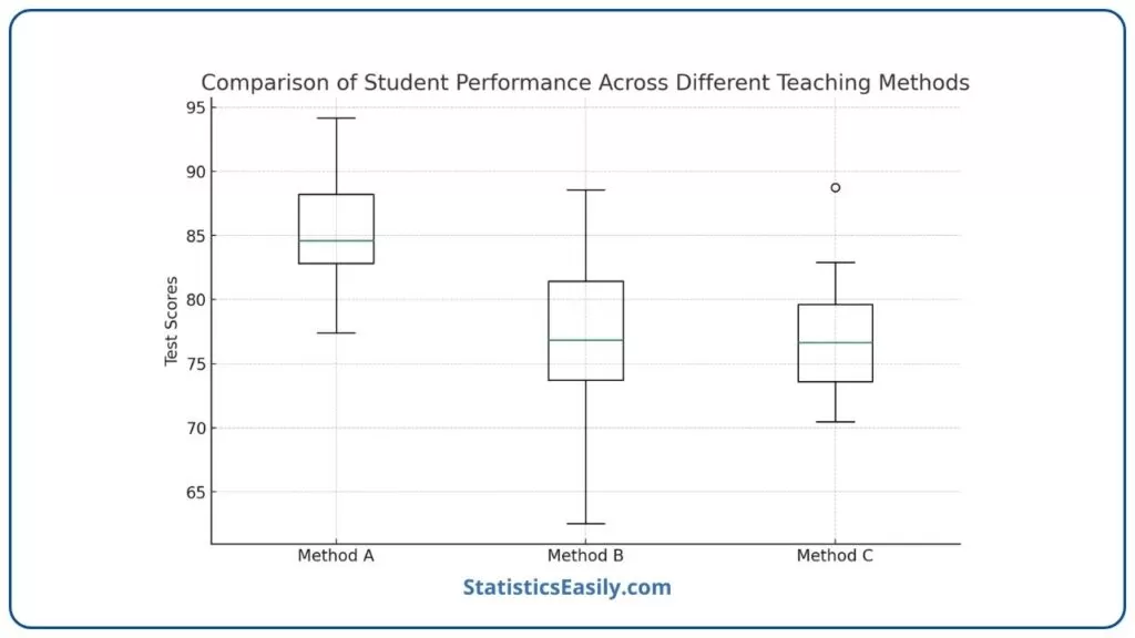
Box Plots: Ideal for visualizing data distribution, medians, quartiles, and outliers. Example: Displaying score distribution for each teaching method.

Tutorial on Creating Graphs in R

Creating a Bar Graph:

library(ggplot2) ggplot(your_data, aes(x=independent_variable, y=dependent_variable, fill=independent_variable)) + geom_bar(stat=”summary”, fun=mean) + geom_errorbar(stat=”summary”, fun.data=mean_se, width=0.2) + labs(x=”Group”, y=”Mean Value”) + theme_minimal() 

Creating a Box Plot:

ggplot(your_data, aes(x=independent_variable, y=dependent_variable, fill=independent_variable)) + geom_boxplot() + labs(x=”Group”, y=”Scores”) + theme_minimal() 

---

Conclusion

Summarizing Key Takeaways from the Guide

The journey through the One-Way ANOVA Statistical Guide has equipped you with a comprehensive understanding of the One-Way ANOVA test. Key takeaways include:

• One-way ANOVA is a robust statistical method for comparing means across multiple independent groups.
• It’s essential to ensure the differences observed are not due to chance but indicate a real effect.
• The test’s assumptions — normality, homogeneity of variances, and independence of observations — are crucial for the validity of its results.
• Reporting results accurately involves presenting the F-statistic, degrees of freedom, p-values and effect sizes, as well as ensuring that the interpretation aligns with the research context.
• Graphical representation of results should be clear and informative, aiding in the communication of data findings.

Encouraging Best Practices in Statistical Analysis

As researchers, it is imperative to uphold the highest standards of statistical analysis. This includes:

• Diligently checking assumptions before proceeding with ANOVA.
• Choosing appropriate post hoc tests based on your specific data conditions.
• Reporting and interpreting results precisely and about the overarching research question.
• Continuously seeking to enhance your statistical skills and knowledge.

Final Thoughts and Additional Resources

Mastering One-Way ANOVA opens a realm of possibilities for data analysis, enabling researchers to unveil insights that drive their fields forward. While this guide has provided a foundational framework, the journey of learning and discovery is ongoing.

Explore resources such as advanced statistical textbooks, online courses, and peer-reviewed journal articles to further your expertise. Engage with communities of practice, attend workshops, and collaborate with statisticians to enrich your analytical acumen.

---

Recommended Articles

Delve deeper into data analysis and elevate your research capabilities with our curated selection of in-depth statistical guides. Expand your knowledge, refine your skills, and stay at the forefront of statistical excellence.

1. ANOVA vs MANOVA: A clear and concise guide
2. ANOVA and T-test: Understanding the Differences
3. ANOVA versus ANCOVA: Breaking Down the Differences

---

Frequently Asked Questions (FAQs)

Q1: What exactly is One-way ANOVA? One-way ANOVA, or Analysis of Variance, is a statistical test used for comparing the means of three or more independent groups to see if they are statistically significantly different. It’s a vital tool in experiments exploring group differences under different treatments or conditions.

Q2: When should One-way ANOVA be used? It’s ideal for situations where you need to compare the means of more than two independent groups. For example, it can be used in medical research to compare patient responses to different medications.

Q3: What are the assumptions behind One-way ANOVA? The test assumes that the data is normally distributed within each group, the variances across groups are equal (homogeneity of variances), and the observations are independent.

Q4: What is an F-statistic in ANOVA? The F-statistic in ANOVA is a calculated ratio used to determine if there are significant differences between the group means. It compares the variance between groups to the variance within groups. A higher F-statistic can indicate a significant difference.

Q5: Why can’t I use multiple t-tests instead of ANOVA? Using multiple t-tests for comparing more than two groups increases the risk of a Type I error – falsely finding a difference when there is none. ANOVA controls this error rate across all group comparisons.

Q6: How do I interpret a significant ANOVA result? A significant result, indicated by a p-value less than your threshold (usually 0.05), suggests that at least one group’s mean differs from the others. Post hoc tests are then used to determine specifically which groups differ.

Q7: Are there non-parametric alternatives to One-way ANOVA? Yes, the Kruskal-Wallis H Test is a non-parametric alternative that is used when data does not meet the normality assumption of ANOVA. It’s useful for ordinal data or non-normally distributed interval data.

Q8: Can One-way ANOVA be used for repeated measures? No, One-way ANOVA is not suitable for repeated measures. A repeated measures ANOVA or a mixed model approach is more appropriate for such designs.

Q9: How does homogeneity of variances affect ANOVA? Unequal variances can affect the accuracy of the F-statistic in ANOVA, leading to incorrect conclusions. If this assumption is violated, it’s crucial to test for homogeneity of variances and use alternative methods like Welch’s ANOVA.

Q10: What should I do if my data doesn’t meet ANOVA assumptions? If the assumptions are not met, consider data transformation techniques to meet normality, use robust ANOVA methods for unequal variances, or explore non-parametric tests like the Kruskal-Wallis test for non-normal distributions.