Pearson Correlation Coefficient Statistical Guide

You will learn the intricacies of interpreting r-values and their profound impact on data correlation analysis with our Pearson Correlation Coefficient Statistical Guide.

Introduction

At the heart of statistical analysis lies the Pearson Correlation Coefficient (r) — a fundamental tool for quantifying the strength and direction of a linear relationship between two continuous variables.

Whether in scientific research, data science, or economic forecasting, the Pearson Correlation Coefficient stands as a pivotal measure, offering insights into the degree to which two variables move in unison.

Far from being a mere mathematical abstraction, ‘r’ reflects the nuanced interplay between datasets, guiding analysts in uncovering the underlying patterns within the fabric of complex data structures.

This statistical guide will dissect the Pearson Correlation Coefficient, elucidating its calculations, interpretations, and the critical assumptions underpinning its use.

Highlights

The Pearson r quantifies linear relationships between variables ranging from +1 to -1.
Values of r closer to +1 or -1 indicate stronger linear associations in datasets.
The Pearson correlation coefficient remains unaffected by different units of measurement.
Assumptions of linearity and homoscedasticity are crucial for Pearson’s r validity.
Pearson’s r doesn’t imply causality, only the degree of linear correlation.

Understanding the Pearson Correlation Coefficient (r)

The Pearson Correlation Coefficient (r) is the statistical standard for measuring the degree of linear relationship between two variables. This coefficient provides a numerical summary ranging from -1 to +1, where each endpoint represents a perfect linear relationship, either negative or positive. An ‘r’ value of 0 indicates no linear correlation between the variables. It reflects how much one variable can predict another through a linear equation. In practice, the value of ‘r’ guides analysts in determining the predictability and strength of the relationship, offering a foundation for further statistical modeling and inference.

Understanding ‘r’ is pivotal for fields that rely on data analysis to make informed decisions, from healthcare research to financial forecasting. Its calculation involves comparing the variance shared between the variables to the product of their variances, thus encapsulating the essence of their synchronous fluctuations.

Visual Aid

To exemplify, consider a dataset examining the relationship between hours of study and exam scores. We expect to see a positive correlation; as the hours of study increase, so should the exam scores. This would be depicted as a collection of upward points on a scatter plot.

Conversely, suppose we were to look at the number of hours spent on leisure activities and exam scores. In that case, we might find a negative correlation, illustrated by a downward trend.

The points would display no discernible pattern or direction in a scenario with no correlation, such as the relationship between shoe size and exam scores.

Below is a visual representation of these scenarios:

Positive Correlation: As one variable increases, so does the other.
Negative Correlation: As one variable increases, the other decreases.
No Correlation: No discernible linear pattern in the relationship between variables.

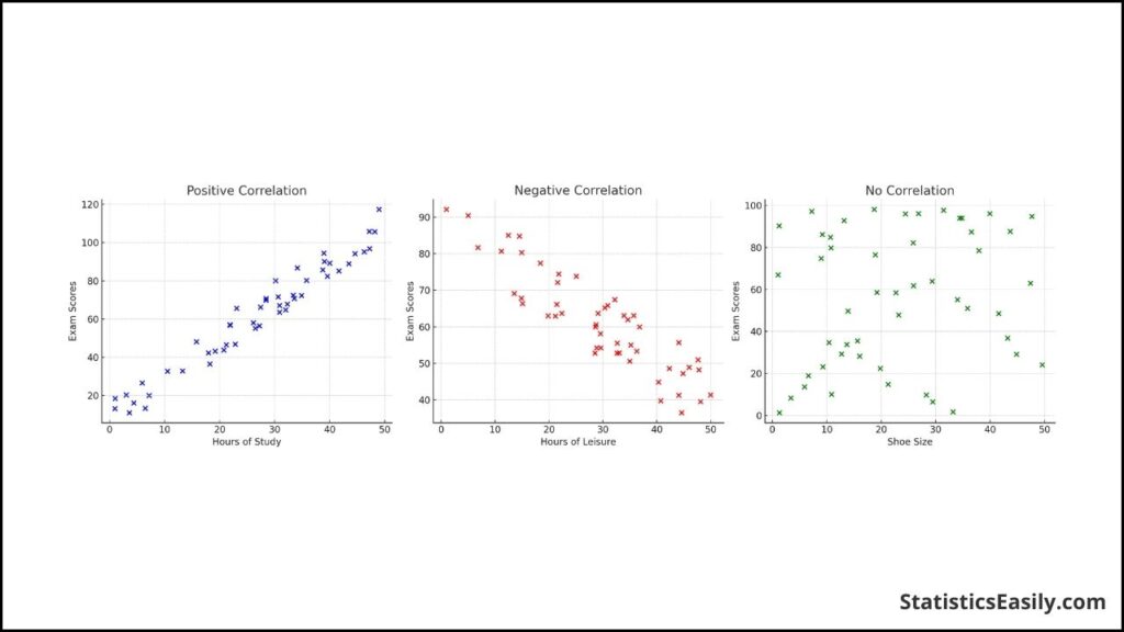
This graph is a powerful tool in the preliminary analysis, allowing for a rapid assessment of potential relationships worth investigating with more sophisticated statistical techniques.

The Range of Values and What They Indicate

The Pearson Correlation Coefficient (r) encapsulates the strength and direction of a linear relationship between two variables, with its values always lying between -1 and +1. The extremities of this range signify perfect correlations: +1 denotes a perfect positive linear correlation, where variables move precisely in tandem, while -1 indicates a perfect negative linear correlation, with one variable increasing as the other decreases. An ‘r’ value at 0 implies no linear correlation; the variables do not show linear dependency.

This range is crucial for understanding the dynamics between variables. For example, an ‘r’ value close to +1 suggests that an increase in one variable will likely be accompanied by an increase in the other to a similar extent. Conversely, an ‘r’ value close to -1 indicates that an increase in one is typically associated with a decrease in the other. The closer the value is to 0, the weaker the linear relationship, signifying that variations in one variable do not reliably predict changes in the other.

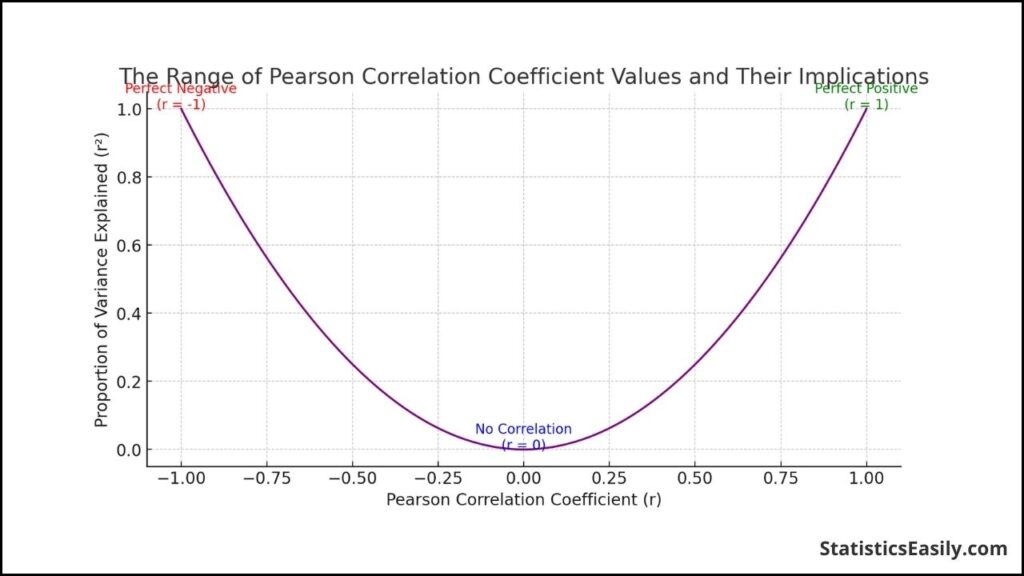
The Coefficient of Determination (r²)

After understanding ‘r’, the coefficient of determination, denoted as ‘r²’, becomes an essential metric. It represents the squared value of ‘r’. It indicates the proportion of the variance in the dependent variable that is predictable from the independent variable. Essentially, ‘r²’ gives us the percentage of how much one variable explains the other.

For instance, if ‘r’ is 0.8, squaring it to get ‘r²’ gives 0.64. This means the variance in the other variable accounts for 64% of the variance in one variable. It’s a powerful way to quantify the predictive power of the linear model created by the two variables. When ‘r²’ is high, the model’s predictions based on the linear relationship will likely be more accurate.

The graphical representation illustrates this relationship, illustrating how the value of ‘r’ correlates with the explained variance. This gives a visual and intuitive understanding of how ‘r²’ functions as a determinant of correlation strength.

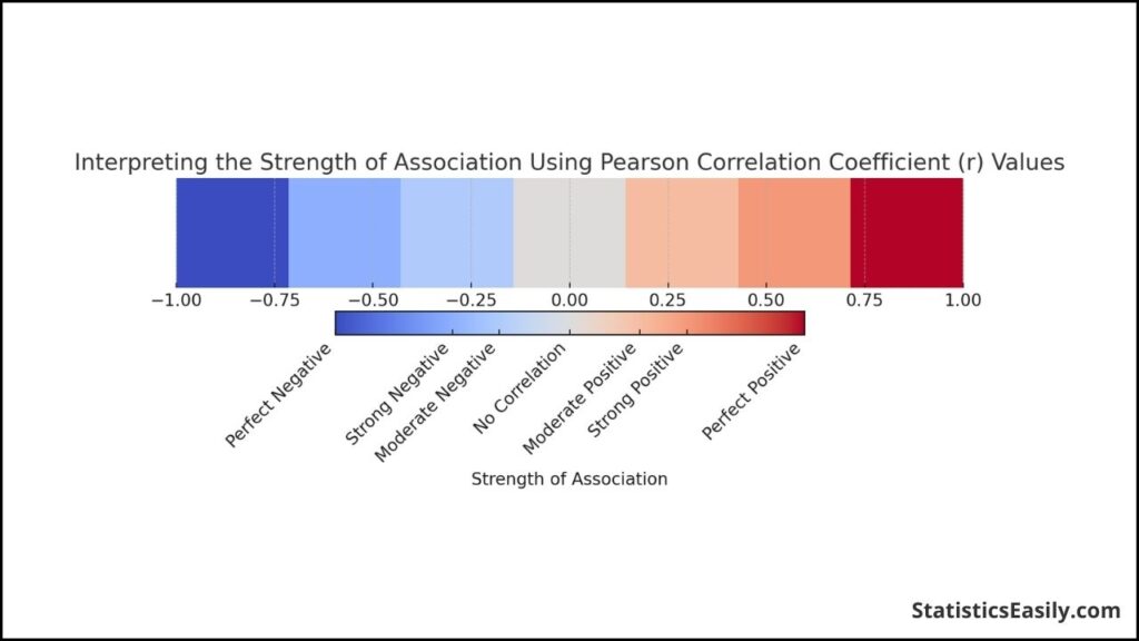
Strength of Association: Interpreting ‘r’ Values

The strength of association between two variables, as indicated by the Pearson correlation coefficient ‘r’, measures how closely data points conform to a linear pattern. When interpreting ‘r’ values, several thresholds are commonly used to describe the strength of the relationship qualitatively:

Perfect: An ‘r’ value of -1 or +1 means that the data points lie precisely on a line; in other words, the two variables are in perfect linear association.
Strong: ‘r’ values closer to -1 or +1 (but not perfect) suggest a strong linear relationship with little deviation from the line.
Moderate: ‘r’ values further from the extremes (around -0.5 to 0.5) indicate a more moderate linear association.
Weak or None: When ‘r’ is close to 0, it suggests a weak or no linear association; the variables appear to have no linear relationship.

The accompanying graphical representation maps ‘r’ values to a color spectrum where the extremes (red for negative and blue for positive) represent stronger associations, and the midpoint (white) represents no association.

Variable Types Suitable for Pearson’s r

The Pearson correlation coefficient is designed to measure the linear relationship between two variables that are both continuous and on an interval or ratio scale. Continuous variables can take on infinite values within a given range, like temperature, height, weight, or test scores.

Interval variables are numerical values where the order and the exact difference between values are meaningful, such as temperature in Celsius or Fahrenheit.

Ratio variables: These have all the properties of interval variables and a clear definition of zero. Examples include weight in kilograms or age in years.

Variables that are not suitable for Pearson’s r include:|

Nominal variables: These are categorical data that do not have a numerical value or order, such as gender, race, or the presence or absence of a condition.

Ordinal variables: While they involve order, the intervals between the values are not uniform or known. An example is a Likert scale (e.g., a 1 to 5 rating).

It’s essential to ensure that the data do not violate the assumptions of Pearson’s correlation, such as the assumption of linearity, the presence of outliers, and homoscedasticity (equal variances along the line of best fit).

Unit Measurement and Its Irrelevance to ‘r’

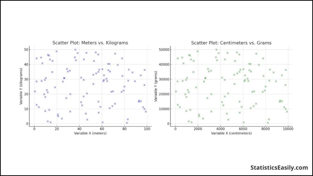
The Pearson correlation coefficient, ‘r’, is a dimensionless measure. This means that it does not depend on the units of measurement of the variables involved. Instead, it quantifies the strength and direction of the linear relationship between two variables. Consequently, whether you measure these variables in meters or centimeters, kilograms or grams, does not affect the value of ‘r’.

For instance, if you have two variables, Variable X measured in meters and Variable Y measured in kilograms, and you calculate ‘r’, you would get the same value as if you measured Variable X in centimeters and Variable Y in grams. This is because the formula for ‘r’ standardizes the variables by their standard deviations, effectively removing the units from the equation.

In our example, the calculation of ‘r’ for the variables in meters and kilograms resulted in a correlation of approximately -0.0661. When we converted these variables to centimeters and grams and recalculated ‘r’, we obtained the same correlation value of approximately -0.0661. This demonstrates the irrelevance of units to the Pearson correlation coefficient, ensuring that the measure of association remains consistent regardless of the scales used for measurement.

This property is particularly useful in research and analysis, allowing for the direct comparison of results across studies that may use different measurement units. It also simplifies the interpretation of correlation, focusing on the relationship itself rather than the specific magnitudes of change.

Independent and Dependent Variables: The Impartiality of ‘r’

A notable characteristic of ‘r’ is its impartiality regarding categorizing variables as dependent or independent.

When calculating ‘r’, the focus is on the direction and strength of the linear association, not on which variables are the cause or effect. This impartiality makes ‘r’ a robust metric applicable across various contexts regardless of the nature of the variables involved.

The Neutrality of ‘r’ in Action

To illustrate, let’s consider a study examining the relationship between the amount of fertilizer used (in kilograms) and the crop yield (in tons). Suppose we designate the amount of fertilizer as the independent variable and the crop yield as the dependent variable and compute ‘r’. In that case, we obtain a value reflecting this linear association’s strength.

Interestingly, if we reverse the roles of the variables, treating the crop yield as independent and the amount of fertilizer as dependent, the value of ‘r’ remains unchanged. This exemplifies that ‘r’ is unaffected by the functional dependency of the variables; it merely quantifies the linear relationship between them.

To visualize this impartiality, consider the following diagram:

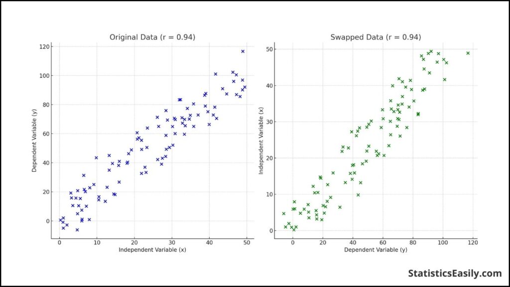
In the diagram, two scatter plots represent the same linear relationship with the variables swapped. In both plots, the line of best fit is identical, and the calculated value of ‘r’ is the same. This serves as a visual reminder that regardless of which independent or dependent variable, ‘r’ provides a consistent measure of the linear relationship.

The Assumptions Behind Pearson’s Correlation

The Pearson correlation coefficient (r) is valid under specific conditions. Here, we discuss the seven critical assumptions required:

Continuous Scale: Both variables must be measured on a continuous scale. Continuous data can take on any value within a range and are not restricted to categories or discrete values.

Paired Observations: The data for the two variables should be paired. Each observation in one variable corresponds to an observation in the other variable.

Independence of Observations: Each pair of observations should be independent of all other pairs. The value of one pair does not depend on the value of another.

Linear Relationship: There must be a linear relationship between the two variables. This means that as one variable increases or decreases, the other variable also increases or decreases in a manner that a straight line can represent.

Bivariate Normal Distribution: Ideally, both variables should be normally distributed, and the pairs of variables should follow a bivariate normal distribution.

Homoscedasticity: The data points around the regression line should be consistently spread out at every level of the independent variable, meaning the variance within each variable is constant.

No Outliers: The data should not contain any significant outliers because they can disproportionately affect the correlation coefficient’s value.

By meeting these assumptions, the Pearson correlation coefficient can be a reliable measure of association between two continuous variables, reflecting the degree of linear relationship. The visual aids can serve as a diagnostic tool to ensure these assumptions are met.

Detecting and Managing Outliers

Outliers can distort the true relationship between two variables in several ways:

Increase or Decrease in r: An outlier can artificially inflate or deflate the correlation coefficient, giving a false impression of a stronger or weaker linear relationship than actually exists.
Misleading Interpretation: Outliers can cause a non-linear relationship to appear linear or obscure a significant relationship, leading to incorrect conclusions.

Methods for Detecting Outliers

Detecting outliers involves both graphical and statistical methods:

Graphical Methods: Scatter plots are invaluable for visually inspecting the data for outliers. Points falling far from the main data cluster can be considered potential outliers.
Statistical Methods: Techniques like the Z-score, where values more than 3 standard deviations from the mean are often considered outliers, and the Interquartile Range (IQR) method, where values outside 1.5 times the IQR from the quartiles are outliers, are commonly used.

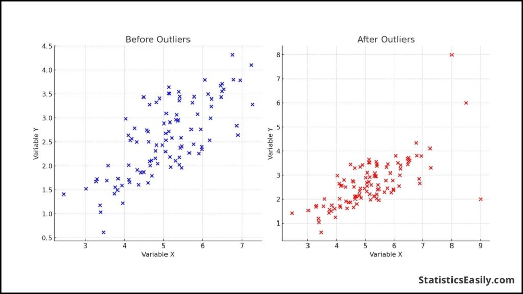
Pearson Correlation Coefficient Statistical Guide

Before Outliers: The left plot shows a relatively linear relationship between variables X and Y, indicating a potential positive correlation without outliers. After Outliers: The right plot introduces outliers to the dataset, visibly distorting the perceived relationship between X and Y, which could significantly affect the Pearson correlation coefficient r.

Managing Outliers

Once detected, outliers can be managed through various approaches:

Exclusion: Removing outliers from the analysis, which is appropriate if the outliers are errors or not representative of the population.
Transformation: Applying a mathematical transformation, such as logarithmic or square root transformations, to reduce the skewness caused by outliers.
Imputation: Replacing outlier values with more representative values, such as the mean or median of the data, though this can potentially bias the results.

Reporting Pearson Correlation Results

When you report the results of a Pearson correlation analysis, you should include the following:

Correlation Coefficient (r): This is the primary result of your analysis, indicating the strength and direction of the linear relationship between the two variables.

Degrees of Freedom (df): This is calculated as the number of pairs of scores minus 2 (N−2). It is used in significance testing.

P-Value: This indicates whether the observed correlation is statistically significant. A standard threshold for significance is p < 0.05, but this can vary depending on the field and specific research context.

Confidence Interval: While not always included, the confidence interval for r provides a range within which the true correlation coefficient will likely fall.

Narrative Explanation: Alongside the numerical results, a brief interpretation of what the correlation coefficient means in the context of your study is helpful.

Example Report

Here’s an illustrative example of how to report Pearson correlation results in a research paper or analysis report:

“A Pearson correlation analysis was conducted to examine the relationship between hours of study and exam scores among university students. The results indicated a strong, positive correlation between the two variables, r(98) = 0.76, p < .001. This suggests that increased study hours are associated with higher exam scores. The strength of this relationship is considered robust, as indicated by the high correlation coefficient and the significant p-value.“

Key Points to Remember

Always report the exact value of r and the p-value.
Interpret the results in the context of your study, explaining what the correlation means for your specific research question.
Be cautious not to imply causation from correlation. A high or low r value indicates only the strength and direction of a linear relationship, not that one variable causes changes in the other.
Consider discussing any potential limitations or factors that might affect the interpretation of the correlation, such as the presence of outliers or the assumption of linearity.

By following these guidelines, you ensure that your reporting of Pearson correlation results is clear, comprehensive, and valuable for your audience, contributing effectively to the broader scientific dialogue.

Statistical Significance and the Coefficient of Determination (r²)

Understanding the statistical significance and the coefficient of determination (r²) is essential when interpreting the results of a Pearson correlation analysis. These concepts help determine the strength and direction of the linear relationship between two variables and the reliability and explanatory power of the correlation observed.

Statistical Significance

Statistical significance in the context of a Pearson correlation indicates the likelihood that the observed correlation between two variables is not due to random chance. The p-value associated with a Pearson r indicates whether the observed correlation is statistically significant.

Interpretation: A common threshold for statistical significance is p < 0.05, meaning there’s less than a 5% probability that the observed correlation occurred by chance. However, the threshold can vary based on the study’s context or discipline.

Reporting: When reporting statistical significance, include the exact p-value. For example, “The correlation between variable X and Y was significant, r(48) = 0.62, p=0.003.“

Coefficient of Determination (r²)

The coefficient of determination, r², is obtained by squaring the Pearson correlation coefficient (r). It represents the proportion of the variance in one variable that is predictable from the other variable.

Interpretation: An r² value of 0.36, for example, suggests that the variance in the other variable explains 36% of the variance in one variable. The higher the r², the stronger the explanatory power of the linear relationship.

Contextual Relevance: r² provides a more intuitive understanding of the correlation’s strength by quantifying how much of the change in one variable is associated with changes in the other.

Example of Reporting r²

“In our analysis, the Pearson correlation coefficient between hours studied and exam scores was r = 0.60, statistically significant with p < 0.001. Squaring this correlation coefficient to calculate the coefficient of determination (r²), we find r² = 0.36. This indicates that 36% of the variability in exam scores can be explained by the amount of time spent studying. Such a finding highlights the substantial impact of study hours on exam performance.“

Conclusion

In this comprehensive guide, we have explored the intricacies of the Pearson Correlation Coefficient (r), a foundational tool in statistical analysis for measuring the linear relationship between two continuous variables. From scientific research to economic forecasting, r serves as a pivotal metric, shedding light on the synchronization of variables and guiding the discovery of underlying data patterns.

Key takeaways include:

Pearson’s r Range: The Pearson r value ranges from +1 to -1, where values close to the extremes indicate strong linear associations and a value of 0 signifies no linear correlation.
Interpretation of r: The value of r quantifies the direction and strength of a linear relationship, enabling predictions and insights into variable interdependencies.
Statistical Significance: The significance of r, determined by the p-value, assesses whether the observed correlation is likely not due to chance.
Coefficient of Determination (r²): Squaring r yields r², which explains the percentage of variance in one variable predictable from the other, enhancing the interpretability of the correlation’s impact.
Assumptions for Validity: The valid application of Pearson’s r requires adherence to assumptions such as linearity, homoscedasticity, and the absence of outliers, ensuring reliable results.
Outlier Management: Identifying and addressing outliers is crucial, as they can significantly skew r, affecting the correlation’s accuracy and interpretation.

The Pearson Correlation Coefficient transcends mere numerical analysis, offering a window into the elegant dance of variables within datasets. It compels researchers and analysts to delve deeper into the fabric of their data, uncovering relationships that inform theories, drive discoveries, and guide decision-making.

Frequently Asked Questions (FAQs)

Q1: What exactly is the Pearson Correlation Coefficient? It’s a statistical measure that reflects the linear relationship between two continuous variables, denoted by r.

Q2: When is it appropriate to use Pearson’s r? Use Pearson’s r to measure the strength and direction of a linear relationship between two variables.

Q3: Can Pearson’s r determine causality between variables? No, Pearson’s r can only indicate the strength of a linear association, not a cause-and-effect relationship.

Q4: How does the scale of measurement affect Pearson’s r? It doesn’t; Pearson’s r is scale-invariant, meaning it’s not affected by the units of measurement of the variables.

Q5: What does a Pearson r value of 0 indicate? An r value of 0 suggests no linear correlation between the variables being studied.

Q6: Are there assumptions underlying the use of Pearson’s r? Yes, the data should be normally distributed, linearly related, and homoscedastic, among other things.

Q7: What is the range of values for Pearson’s r? Pearson’s r can range from +1, indicating a perfect positive correlation, to -1, a perfect negative correlation.

Q8: How do outliers affect Pearson’s r? Outliers can significantly skew the results, making the correlation appear stronger or weaker than it is.

Q9: Can Pearson’s r be used for ordinal data? No, Pearson’s r is not suitable for ordinal data. Spearman’s rank correlation is typically used instead.

Q10: How do you report Pearson correlation results? To determine statistical significance, report the r-value, degrees of freedom, and p-value.

Pearson Correlation Coefficient Statistical Guide

Introduction

Highlights