Generalized Linear Model (GLM) Distribution and Link Function Selection Guide

You will learn to select the Generalized Linear Model Distribution and Link Function for optimal modeling accuracy.

---

Introduction

Generalized Linear Models (GLMs) represent an extension of traditional linear regression models designed to accommodate a wide array of data types and distribution patterns. This flexibility makes GLMs indispensable in the arsenal of data scientists and statisticians. At their core, GLMs consist of three principal components:

• The random component specifies the probability distribution of the response variable;
• The systematic component relates the predictors to the response through a linear predictor function;
• The link function connects the distribution’s mean with the linear predictor.

Selecting an appropriate Generalized Linear Model Distribution and Link Function is not merely a technical decision; it’s an art that enhances the model’s accuracy and predictive performance. Understanding how to match the distribution and link function with the data’s inherent characteristics is pivotal for unlocking the full potential of GLMs, leading to more insightful and reliable analyses. This guide aims to illuminate the path toward optimal model configuration, ensuring your GLM harnesses the true essence of your data.

---

Highlights

• Choosing the correct GLM distribution significantly enhances model precision.
• Link functions transform model predictions to the scale of the response variable.
• Binomial distribution with a logit link is ideal for binary outcome data.
• Model fit improves by matching distribution to the data’s nature.
• Iteratively testing link functions can unveil the best model performance.

---

Understanding GLM Distribution

Generalized Linear Models (GLMs) are a cornerstone in statistical analysis, accommodating a broad spectrum of data types through their adaptable framework. Central to their utility is the concept of GLM distribution, which allows these models to transcend the limitations of traditional linear regression by embracing distributions beyond the normal. This section delves into the various distributions underpinning GLMs. It guides you in aligning your data with the most suitable GLM distribution.

Diverse Distributions for Varied Data Types

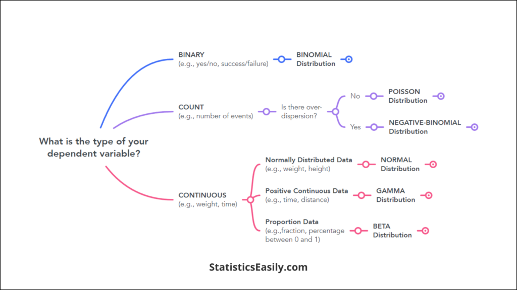
GLMs are uniquely designed to handle different data distributions, each catering to specific types of response variables. The Binomial distribution is frequently employed for binary outcomes, such as success/failure scenarios. In contrast, the Poisson distribution is pivotal for counting data, addressing “how many?”. For continuous data that adheres to positive values, the Gamma distribution offers a fitting model. Each distribution is tailored to capture the essence of the underlying data structure, ensuring that the model’s assumptions align with the data’s natural behavior.

Tailoring the Model to Your Data

Selecting the proper GLM distribution is not a one-size-fits-all process but a nuanced decision that significantly impacts model accuracy and interpretability. The key lies in understanding your data’s distribution and its inherent characteristics. For instance, the Poisson distribution might be your starting point if your data represents counts or rates. Conversely, the Binomial distribution could be more appropriate for binary or proportion data. This selection process is critical, as it ensures that the GLM reflects the real-world processes generating your data, enhancing the model’s predictive capabilities and interpretability.

By thoughtfully matching your data with the correct GLM distribution, you elevate the analytical rigor of your study, paving the way for more precise and meaningful insights. This foundational step is instrumental in harnessing the full potential of GLMs, enabling them to articulate the intricate stories hidden within your data.

---

The Role of Link Functions in GLMs

Link functions are the linchpins in Generalized Linear Models (GLMs), serving as the critical bridge between the linear predictors and the response variable’s expected value. Their role cannot be overstated, as they enable modeling a wide range of data types beyond the capabilities of traditional linear regression. By transforming the predictions to the scale of the response variable, link functions ensure that the model’s outputs adhere to the appropriate data range and distribution, thereby enhancing the interpretability and accuracy of the model’s predictions.

Transforming Predictions to Reality: The Essence of Link Functions

Link functions are not one-size-fits-all; they are carefully selected based on the response variable’s nature and the distribution chosen for the GLM. Standard link functions include the logit function, widely used in logistic regression for binary data, transforming probabilities into an unbounded continuous scale. The identity link, inherent to normal distribution models, assumes a direct relationship between the predictors and the response variable. The log link is typical for counting data modeled with a Poisson distribution, ensuring the model’s predictions remain positive and continuous.

Applications of Link Functions: From Theory to Practice

The choice of link function has profound implications for the model’s application and interpretation. For instance, in epidemiology, the logit link in logistic regression models the odds of an event occurring, such as disease presence or absence. In economics, the identity link in linear regression models directly predicts quantitative outcomes like income based on predictors like education and experience. Meanwhile, in insurance, the exponential link in Poisson regression models claims counts, ensuring predictions are non-negative and discrete.

By adeptly selecting and applying the appropriate link function, statisticians and data scientists can craft GLMs that capture the underlying patterns in their data and convey their findings in an accurate and intuitively understandable manner to their audience. This section of the guide demystifies the selection and application of link functions, providing you with the knowledge to enhance the precision and interpretability of your GLMs.

---

Selecting the Right Distribution and Link Function

Selecting the appropriate Generalized Linear Model Distribution and Link Function is paramount to the success of your statistical analysis. The nature of your response variable and the relationship between the response and the predictors guide this selection. Here, we provide a detailed guide to help you navigate this critical process.

Step 1: Identifying the Type of Response Variable

The first step in choosing the proper distribution is to identify the type of data you are working with clearly:

• Binary Data: For outcomes that fall into one of two categories (e.g., success/failure, yes/no), the Binomial distribution is the go-to choice. This distribution models the number of successes in a series of independent trials.
• Count Data: The Poisson distribution is typically used when dealing with countable occurrences (e.g., the number of events in a given time or space). It is ideal for data that represent counts and are non-negative integers.
• Continuous Data: The Gamma distribution is often suitable for data taking on any value within a range, especially positive numbers such as durations or amounts. It is used for modeling positively skewed data.
• Normally Distributed Data: When your data approximately follows a normal distribution, especially in the case of continuous outcomes that can take both positive and negative values, the Normal distribution can be applied within the GLM framework.

Step 2: Understanding the Relationship Between Variables

The link function connects the linear predictor to the mean of the response distribution. It should be chosen based on how you expect changes in your predictors to influence the response variable:

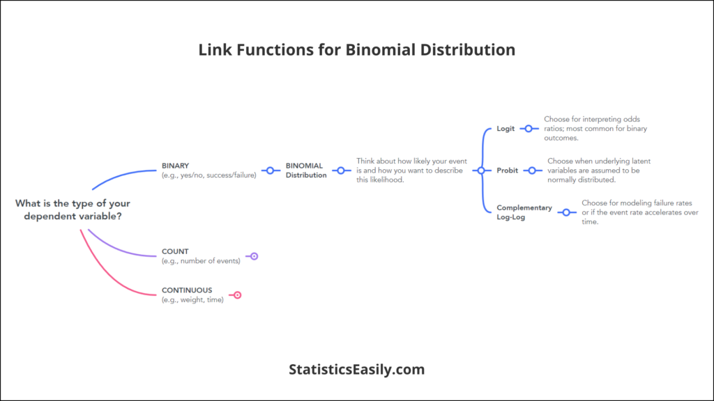
• For Binary Data: The Logit link function is commonly used, transforming the linear combination of predictors to lie between 0 and 1, thus representing probabilities.
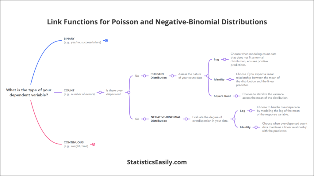
• For Count Data: The Log link function is a natural choice, especially with Poisson distribution, ensuring that predictions are always positive and well-suited for count data.
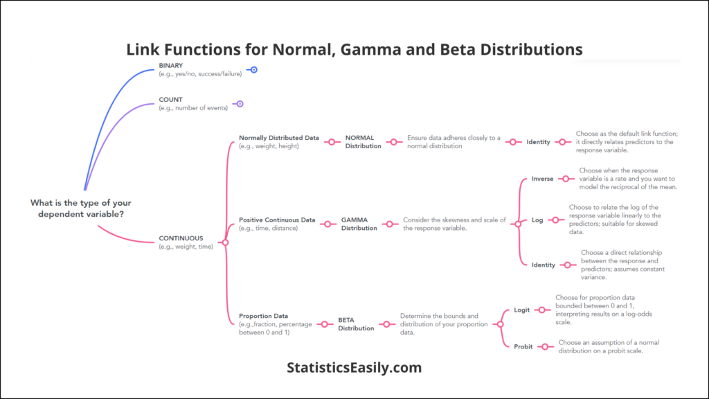
• For Continuous Data with Positive Skew (Gamma): The Inverse link function can be handy when modeling rates or times, ensuring positive predictions.
• For Normally Distributed Data: The Identity link function, which implies a direct relationship between the predictors and the response variable, is often used. This straightforward function implies that the expected value of the response is equal to the linear predictor.

Step 3: Applying Model Diagnostics

After selecting a preliminary distribution and link function based on the above criteria, it’s crucial to validate your choice through model diagnostics:

• Residual Analysis: Examine residuals for patterns that might suggest a poor fit, indicating the need for a different distribution or link function.
• Goodness-of-Fit Tests: Utilize tests such as Deviance or AIC to assess how well your model fits the data quantitatively. These tests can guide you in comparing different models or configurations to find the best fit.

Iterative Refinement

The process of selecting the proper distribution and link function is often iterative. Based on diagnostics, you might need to revisit your choices, trying different distributions or link functions until the diagnostics indicate a good fit.

Following these detailed steps, you will be better equipped to select the most appropriate distribution and link function for your GLM, enhancing the model’s accuracy and interpretability.

Response Variable Type	Suggested Distribution	Common Link Functions	Use Case
Binary Outcome (e.g., success/failure)	Binomial	Logit, Probit, Complementary Log-Log	Modeling probabilities of binary outcomes, such as presence/absence of a disease.
Count Data (e.g., number of events)	Poisson	Log, Identity, Square Root	Counting occurrences in fixed intervals, such as the number of calls received by a call center per hour.
Count Data with Overdispersion	Negative Binomial	Log, Identity	Count data that exhibit variability exceeding Poisson assumptions, such as the number of insurance claims per client.
Continuous Proportions	Beta	Logit, Probit	Proportions that vary between 0 and 1, such as the fraction of an area affected by a certain condition.
Positive Continuous Data	Gamma	Inverse, Log, Identity	Modeling waiting times or service times, where the response variable is always positive.
Normally Distributed Data	Normal (Gaussian)	Identity	Continuous outcomes that are symmetrically distributed, such as test scores or heights.

---

Practical Tips for GLM Optimization

Implementing Generalized Linear Models (GLMs) effectively in R and Python involves understanding the nuances of these powerful tools. By appropriately leveraging the Generalized Linear Model Distribution and Link Function, you can refine your models to achieve higher accuracy and better interpretability. Here are some practical tips to guide you in this process:

Best Practices for Implementing GLMs in R:

1. Use the ‘glm()‘ function: R’s ‘glm()‘ function is versatile, allowing you to specify the model formula, distribution family, and link function. For example, ‘glm(response ~ predictors, family=binomial(link=”logit”), data=mydata)‘ will fit a logistic regression model.

2. Diagnostics with ‘plot()‘ and ‘summary()‘: After fitting your model, use ‘summary(glm_model)‘ to get a detailed summary of model coefficients, significance levels, and more. The ‘plot(glm_model)‘ function can provide diagnostic plots to assess fit and check for assumptions.

3. Model selection with AIC: Use the ‘step()‘ function to perform stepwise model selection based on the Akaike Information Criterion (AIC), helping you to choose a model that balances complexity with goodness of fit.

4. Cross-validation: For model validation, consider using packages like ‘caret‘ or ‘cv.glm()‘ from the boot package to perform cross-validation and assess the model’s predictive performance.

Best Practices for Implementing GLMs in Python:

1. Leverage ‘statsmodels‘ or ‘scikit-learn‘: Python offers multiple libraries for GLM implementation. For a more statistical approach, ‘statsmodels‘ provides detailed summaries and diagnostics. For a machine learning approach, ‘scikit-learn‘ offers simplicity and integration with ML workflows.

2. Model fitting with ‘statsmodels‘: Use ‘statsmodels.api.GLM‘ to fit a GLM, specifying the family and link function. For example, ‘GLM(y, X, family=sm.families.Binomial(sm.families.links.logit)).fit()‘ fits a logistic regression.

3. Diagnostics and validation: Use ‘statsmodels‘ for diagnostic plots and summary statistics. For model validation, consider using ‘sklearn.model_selection‘ for techniques like cross-validation.

4. Feature selection: In ‘scikit-learn‘, you can use regularization techniques available in logistic regression implementations (‘LogisticRegressionCV‘) to perform feature selection and prevent overfitting.

Model Refinement Using Distribution and Link Function:

Iterative refinement: Model building is an iterative process. Start with a simple model and gradually add complexity. Use diagnostics at each step to assess the model’s performance and make informed modification decisions.

Distribution selection: Choose the distribution that best matches the nature of your response variable. For binary outcomes, start with a Binomial distribution; for count data, consider Poisson or Negative Binomial in the case of overdispersion.

Link function choice: The link function should reflect the relationship between the linear predictors and the response scale. For example, use a logit link for probabilities in a Binomial model or a log link for count data in a Poisson model.

Validation and diagnostics: Regularly perform model diagnostics to check for issues such as non-linearity, high leverage points, or heteroscedasticity. Use residual plots, influence plots, and Cook’s distance to identify potential problems.

---

Conclusion

As we conclude our journey through the intricacies of Generalized Linear Model Distribution and Link Function selection, it’s crucial to revisit the pivotal insights that enhance the precision of our statistical models and the depth of our analyses. This guide has illuminated the path toward harnessing the full potential of GLMs, emphasizing the criticality of matching the model components with the inherent characteristics of the data.

Key Takeaways:

Tailored Approach: The essence of GLM optimization lies in the thoughtful selection of the distribution and link function, tailored to the nature of the response variable and the expected relationship with the predictors. From binary outcomes requiring a Binomial distribution paired with a logit link to counting data best modeled by a Poisson distribution and a log link, each choice plays a foundational role in model accuracy.

Diagnostics and Iteration: The journey doesn’t end with the initial selection. Diagnostics are crucial in refining the model, with residual analysis and goodness-of-fit tests guiding iterative adjustments to ensure the best possible model fit.

Real-World Application: The true test of these principles lies in their application to real-world data. The versatility of GLMs allows them to be adapted to a wide array of scenarios, from epidemiological studies predicting disease incidence to econometric models evaluating market trends.

---

Recommended Articles

Explore more insights and advanced techniques in our comprehensive statistical modeling and data analysis articles collection. Dive deeper into the world of data science with our expert guides.

1. Navigating the Basics of Generalized Linear Models: A Comprehensive Introduction
2. Generalized Linear Model (GLM) Distribution and Link Function Selection Guide
3. Understanding Distributions of Generalized Linear Models
4. The Role of Link Functions in Generalized Linear Models

---

Frequently Asked Questions (FAQs)

Q1: What is a Generalized Linear Model (GLM)? A GLM is a flexible generalization of ordinary linear regression that allows response variables to have error distribution models other than a normal distribution.

Q2: Why is choosing the correct distribution important in GLMs? Selecting the appropriate distribution helps accurately model the data, reflecting its underlying structure and variability.

Q3: What are link functions in GLMs? Link functions define the relationship between the linear predictor and the mean of the distribution function.

Q4: How do I select the right link function for my GLM? The choice of link function depends on the nature of the dependent variable and the data distribution.

Q5: Can I use multiple distributions in a single GLM? A single distribution is typically chosen to best fit the data in a GLM, but complex models may integrate various distributions.

Q6: What is the most common distribution used in GLMs? The Binomial distribution is widely used for binary data, while the Normal distribution is typical for continuous data.

Q7: How do diagnostics play a role in GLM distribution and link function selection? Diagnostics help assess the model’s fit, identify the presence of outliers, and guide the selection process.

Q8: Can software tools help select the GLM distribution and link function? Yes, statistical software like R and Python offers packages that facilitate the selection and evaluation of GLMs.

Q9: How does the choice of link function affect model interpretation? The link function influences how model coefficients are interpreted, affecting the clarity and directness of insights.

Q10: Can I change the distribution and link function after model fitting? Yes, model refinement often involves iteratively testing different distributions and link functions to improve fit and accuracy.