Logistic Regression Using R: The Definitive Guide

You will learn the pivotal role of logistic regression using R in predictive analytics and data-driven decision-making.

---

Introduction

In the dynamic field of data science, logistic regression is a pivotal tool for binary classification problems, offering profound insights into data through predictive modeling. This statistical technique, particularly when leveraged using R, a versatile tool renowned for its statistical analysis and modeling capabilities, empowers analysts and researchers to uncover hidden patterns and make informed decisions. The synergy between logistic regression and R equips practitioners with a robust framework to tackle complex data challenges, establishing a foundation for data-driven innovation and strategic insights. This guide aims to illuminate the path for mastering logistic regression using R, ensuring readers are equipped with the knowledge to harness the full potential of this powerful analytical approach.

---

Highlights

• R simplifies complex logistic regression models for better predictive accuracy.
• Logistic regression in R aids in distinguishing binary outcomes efficiently.
• Data preprocessing in R enhances the reliability of the logistic regression model.
• R’s syntax facilitates the intuitive implementation of logistic regression analysis.
• Real-world examples illustrate the practical value of logistic regression using R.

---

Understanding Logistic Regression

Logistic regression is a cornerstone of data science, particularly when solving classification problems with dichotomous outcomes, such as spam or not spam, win or lose, healthy or sick. Unlike linear regression, which predicts outcomes with a continuous range, logistic regression provides a probability score for a given set of features or inputs to fall into a specific category. This makes it invaluable in fields such as medicine for predicting the likelihood of a disease, finance for default likelihood, and marketing for predicting customer behavior.

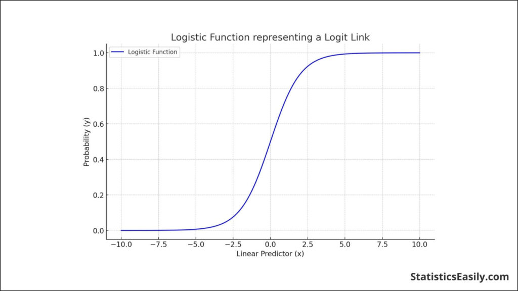
The mathematical foundation of logistic regression lies in the logistic function, often called the sigmoid function. This S-shaped curve can map any real-valued number into a value between 0 and 1, making it perfect for modeling probability scores in binary classification tasks. The equation for logistic regression contrasts with that of linear regression primarily in its use of the logistic function to model the dependent variable. The logistic regression model thus estimates the probability that a given input point belongs to a certain class, which can be expressed mathematically as:

P(Y=1∣X)=1/1+e^{−(β0​+β1​X)}

where P(Y=1∣X) is the probability that the dependent variable Y equals one given the independent variables X, e is the base of the natural logarithm, β0​ is the intercept term, and β1​ represents the coefficient(s) of the independent variable(s) that influence the dependent variable.

In R, logistic regression can be implemented using functions like ‘glm()’ (Generalized Linear Models), with the family set to binomial to specify that it is a binomial logistic regression. The simplicity of this implementation, combined with R’s comprehensive set of tools for data manipulation and analysis, makes logistic regression using R a powerful approach for predictive modeling. Through R’s capabilities, data scientists can preprocess data, build logistic regression models, evaluate their performance, and use them for prediction with relative ease, reinforcing R’s status as a versatile tool in the arsenal of data analysis and modeling.

---

Getting Started with R

Embarking on your journey with R, a language and environment revered for statistical computing and graphics, begins with setting up the necessary foundation. For beginners, the initial step involves installing R, which is straightforward and accessible from the Comprehensive R Archive Network (CRAN). Accompanying R, installing RStudio, a powerful IDE that enhances R’s user experience with its intuitive interface and additional features, is highly recommended.

Upon installation, familiarizing yourself with R’s syntax is paramount for practical data analysis. R’s syntax is unique yet intuitive, allowing users to perform complex data manipulations and analyses with concise code. Key concepts include:

• Variables and Data Types: Understand how to assign values to variables and the various data types in R, such as numeric, character, and logical.
• Vectors and Data Frames: Grasp the creation and manipulation of vectors and data frames, the backbone of data analysis in R.
• Functions and Packages: Learn to use built-in functions and install and load packages, extending R’s capabilities far beyond its base functionality. Packages like ‘glmnet’ and ‘caret’ are invaluable for logistic regression.
• Control Structures: Learn control structures such as if-else statements and loops, which allow you to control the flow of execution in your scripts.

A simple yet illustrative example of R’s syntax in action is the creation and manipulation of a data frame, which might look something like this:

# Create a data frame
my_data <- data.frame(
  Outcome = c("Success", "Fail", "Success", "Fail"),
  Age = c(22, 45, 33, 29),
  Score = c(85, 47, 76, 62)
)

# View the data frame
print(my_data)

# Calculate the mean Score
mean_score <- mean(my_data$Score)
print(paste("Average Score:", mean_score))

This snippet demonstrates variable assignment, data frame creation, and primary function usage. R’s powerful suite of tools and comprehensive approach to data manipulation and analysis make it an essential skill for data scientists and statisticians alike.

---

Preparing Your Data for Logistic Regression

A critical step before applying logistic regression in R is data cleaning and preprocessing. This process ensures that the dataset is formatted correctly, free of errors or irrelevant information, and structured to enhance the performance and accuracy of your logistic regression model.

Data Cleaning involves several vital tasks:

• Handling Missing Values: Use functions like ‘na.omit()’ to remove or ‘impute()’ from the mice package to fill in missing values with estimates.
• Removing Outliers: Outliers can skew results. Techniques like the Interquartile Range (IQR) method can help identify and remove these anomalies.
• Ensuring Data Consistency: Standardize the formatting of your data, such as date formats and categorical values, to avoid inconsistencies.

Data Preprocessing includes:

• Variable Selection: Identify which variables are most relevant to your predicted outcome. This might involve statistical techniques like correlation analysis or domain expertise.
• Data Transformation: Convert categorical variables into dummy variables or factors with functions like ‘factor()’ or ‘model.matrix()’, as logistic regression requires numerical input.
• Feature Scaling: Although not always necessary for logistic regression, standardizing features using scaling functions can sometimes improve model performance.

An illustrative example of preparing your data might involve transforming a categorical variable into a format suitable for logistic regression:

# Assuming 'Gender' is a categorical variable with levels 'Male' and 'Female'
my_data$Gender <- factor(my_data$Gender, levels = c("Male", "Female"))

# Transforming 'Gender' into a dummy variable
my_data <- model.matrix(~ Gender + Age + Score - 1, data = my_data)

This snippet demonstrates converting the ‘Gender’ categorical variable into a dummy variable, a standard step in preparing data for logistic regression. This enables the model to incorporate this information effectively.

The importance of selecting appropriate variables cannot be overstated. Including variables that strongly predict the outcome can enhance model accuracy, while irrelevant variables might dilute the model’s predictive power. Techniques such as backward elimination, forward selection, or even machine learning algorithms like Random Forest can be employed to identify significant predictors.

In sum, careful data preparation paves the way for a robust logistic regression model. It deepens your understanding of the dataset, leading to more insightful and impactful data analysis.

---

Implementing Logistic Regression Using R

Implementing logistic regression in R involves a clear and structured approach. This section will guide you through the steps to perform logistic regression, including code snippets for clarity. The focus will be on how to build the model, interpret its output, and understand the significance of coefficients and model fit.

Step-by-Step Guide

1. Loading the Required Package: To perform logistic regression, ensure that you have the ‘stats’ package, which comes pre-installed with R. This package includes the ‘glm()’ function, essential for logistic regression.

# Ensure the stats package is loaded (it should be by default)
library(stats)

2. Building the Logistic Regression Model: Utilize the ‘glm()’ function, specifying the binomial family to indicate logistic regression. Assume ‘my_data’ is your dataset, ‘Outcome’ is the binary dependent variable, and ‘Predictor1’, ‘Predictor2’ are your independent variables.

# Building the logistic regression model as before
logistic_model <- glm(Outcome ~ Predictor1 + Predictor2, family = binomial, data = my_data)

# Performing a Likelihood Ratio Test
anova(logistic_model, test = "Chisq")

3. Summarizing the Model: To understand the model’s coefficients and their significance, use the ‘summary()’ function.

# Summarizing the logistic regression model
summary(logistic_model)

Interpreting the Output

• Coefficients: The summary output provides coefficients for each predictor. These coefficients represent the log odds for the outcome variable. A positive coefficient indicates that as the predictor variable increases, the log odds of the outcome occurring increase, making the event more likely.
• Significance Levels: Look at the ‘Pr(>|z|)’ column in the summary output. Values here represent the p-value for each coefficient. Typically, a p-value less than 0.05 indicates that the predictor is significantly associated with the outcome variable.
• Model Fit: The summary also includes goodness-of-fit measures. The null and residual deviance indicates how well the model fits the data. A lower residual deviance compared to the null deviance suggests a good fit. Additionally, the Akaike Information Criterion (AIC) measures the model’s quality, where a lower AIC indicates a model that better fits the data without overfitting.

Example Summary Interpretation

Consider the output snippet below from a logistic regression summary:

Coefficients:
            Estimate Std. Error z value Pr(>|z|)
(Intercept)  -1.2345     0.2079  -5.939  3.00e-09 ***
Predictor1     0.4456     0.1102   4.045  5.25e-05 ***
Predictor2    -0.5678     0.1456  -3.900  9.68e-05 ***
---
Signif. codes:  0 ‘***’ 0.001 ‘**’ 0.01 ‘*’ 0.05 ‘.’ 0.1 ‘ ’ 1

(Dispersion parameter for binomial family taken to be 1)

    Null deviance: 234.83  on 170  degrees of freedom
Residual deviance: 144.57  on 168  degrees of freedom
AIC: 150.57

• The ‘Intercept’ and ‘Predictor1’ and ‘Predictor2’ are significant (p < 0.05).
• ‘Predictor1’ has a positive coefficient, suggesting that increasing ‘Predictor1’ increases the log odds of the outcome.
• ‘Predictor2’ has a negative coefficient, indicating that an increase in ‘Predictor2’ decreases the log odds of the outcome.
• The substantial drop in deviance and the AIC value suggests a good model fit.

By following these steps and understanding the model output, you can effectively implement logistic regression in R, paving the way for insightful data analysis and predictive modeling.

---

Enhancing Your Logistic Regression Using R

Improving a logistic regression model’s accuracy and predictive power in R involves several strategic steps, from thoughtful feature selection to advanced model evaluation techniques. Here are some tips and methods to enhance your logistic regression model:

Feature Selection and Transformation

1. Variable Importance: Use techniques like stepwise regression or machine learning algorithms (e.g., Random Forest) to identify the most predictive features for your model. This helps simplify the model by retaining only significant predictors.

library(MASS)
stepwise_model <- stepAIC(logistic_model, direction = "both")
summary(stepwise_model)

2. Dealing with Multicollinearity: High correlation among predictors can distort the significance of variables. Use the Variance Inflation Factor (VIF) to check for multicollinearity and consider removing or combining highly correlated variables.

library(car)
vif(logistic_model)

3. Data Transformation: Non-linear relationships between predictors and the log odds can be captured through transformations like polynomial terms or interaction effects.

logistic_model <- glm(Outcome ~ poly(Predictor1, 2) + Predictor2 + Predictor1:Predictor2, family = binomial, data = my_data)

Model Evaluation Techniques

1. Cross-Validation: Implement k-fold cross-validation to assess the model’s predictive performance on unseen data, which helps in mitigating overfitting.

library(caret)
control <- trainControl(method = "cv", number = 10)
cv_model <- train(Outcome ~ Predictor1 + Predictor2, data = my_data, method = "glm", family = "binomial", trControl = control)

2. Model Performance Metrics: Beyond the AIC and deviance checks, consider ROC (Receiver Operating Characteristic) analysis and calculate the AUC (Area Under the Curve) to evaluate the model’s discriminatory ability between the outcome classes.

library(pROC)
roc_response <- roc(response = my_data$Outcome, predictor = fitted(logistic_model))
auc(roc_response)

3. Residual Analysis: Investigate model residuals to ensure no patterns might suggest poor model fit, such as trends or clusters.

plot(residuals(logistic_model, type = "deviance"))

Enhancing your logistic regression model involves carefully balancing feature engineering, methodical model evaluation, and continuous refinement based on performance metrics. By employing these techniques, you can build a more accurate, robust, and interpretable model that better captures the complexities of your data and provides more reliable predictions.

---

Real-World Applications of Logistic Regression Using R

Logistic regression, mainly when utilized within the R environment, has proven invaluable across a broad spectrum of real-world applications. Its versatility in handling binary outcomes makes it a go-to method for various domains seeking to make informed decisions based on predictive analytics. Here, we delve into practical examples where logistic regression has been successfully applied, shedding light on the insights and implications of its results.

Healthcare and Medicine

In the medical field, logistic regression has been extensively used to predict the likelihood of disease occurrences based on patient data. For instance, by analyzing patient attributes such as age, BMI, and blood pressure, logistic regression models can predict the probability of diabetes onset. This predictive power aids healthcare professionals in identifying high-risk patients, allowing for early intervention and management strategies.

# Predicting diabetes occurrence
diabetes_model <- glm(Diabetes ~ Age + BMI + BloodPressure, family = binomial, data = patient_data)

Financial Services

The banking and finance sectors leverage logistic regression to assess credit risk. By evaluating customer data points like income, credit history, and debt levels, logistic regression helps predict the probability of loan default. This insight is crucial for financial institutions to make informed lending decisions, thereby minimizing risk and optimizing loan approval processes.

# Credit risk assessment
credit_risk_model <- glm(Default ~ Income + CreditHistory + DebtLevel, family = binomial, data = customer_data)

Marketing Analytics

In marketing, logistic regression predicts customer behavior, such as the likelihood of purchasing a product or responding to a campaign. Logistic regression models enable marketers to tailor campaigns more effectively by analyzing historical purchase data and demographic information, enhancing customer engagement, and optimizing marketing strategies.

# Predicting customer purchase behavior
purchase_model <- glm(Purchase ~ Age + Gender + PreviousPurchases, family = binomial, data = sales_data)

Social Sciences

Logistic regression is also used in social science research, particularly in areas like voting behavior analysis or understanding social trends. By examining factors such as age, education, and socio-economic status, logistic regression models provide insights into the likelihood of certain social behaviors, contributing to policy-making and sociological understanding.

# Analyzing voting behavior
voting_model <- glm(Voted ~ Age + EducationLevel + SocioEconomicStatus, family = binomial, data = survey_data)

Implications and Insights

The successful application of logistic regression in these domains underscores its significance in predictive modeling. Quantifying the odds of binary outcomes based on predictor variables allows stakeholders to make evidence-based decisions, enhancing efficiency and effectiveness in their respective fields.

Moreover, the insights from logistic regression analyses can lead to proactive measures, policy formulations, and strategic adjustments across industries. Organizations and professionals can implement targeted interventions by identifying key predictors and understanding their impact on the outcome, fostering positive outcomes and mitigating risks.

Logistic regression using R facilitates a deeper understanding of complex relationships within datasets. It empowers various sectors to harness predictive analytics for informed decision-making, showcasing its invaluable role in advancing data-driven initiatives worldwide.

---

Conclusion

In this comprehensive journey through logistic regression using R, we’ve unveiled this statistical technique’s profound impact and versatility across various fields. From healthcare to finance and social sciences, logistic regression stands as a beacon for those seeking to illuminate the hidden patterns within their data. It offers a predictive lens through which binary outcomes can be forecasted precisely. Mastering logistic regression in R not only arms analysts and researchers with a potent tool for data-driven decision-making but also fosters a deeper appreciation for the art and science of predictive modeling. As we’ve traversed from foundational concepts to advanced applications, the value of logistic regression in crafting informed strategies and interventions has been abundantly clear.

---

Recommended Articles

Explore deeper into the world of data science with our related articles. Dive into more topics to broaden your analytics expertise.

1. Logistic Regression Scikit-Learn: A Comprehensive Guide for Data Scientists
2. Understanding Distributions of Generalized Linear Models
3. What Are The Logistic Regression Assumptions?
4. What Are The 3 Types of Logistic Regression?
5. Logistic Regression Using Scikit-Learn (Story)
6. Mastering Logistic Regression (Story)

---

Frequently Asked Questions (FAQs)

Q1: What is Logistic Regression in R? It’s a statistical method for predicting binary outcomes based on independent variables.

Q2: Why use R for Logistic Regression? R provides comprehensive packages like glm() for efficient and detailed logistic regression analysis.

Q3: How does Logistic Regression differ from Linear Regression? Unlike linear regression, which predicts continuous values, logistic regression predicts binary outcomes (0 or 1).

Q4: What are the prerequisites for performing Logistic Regression in R? Basic knowledge of R programming and statistical concepts is essential for logistic regression analysis.

Q5: How to interpret Logistic Regression output in R? The output includes coefficients, which indicate the relationship between each predictor and the log odds of the outcome.

Q6: What is the role of data preprocessing in Logistic Regression? Preprocessing involves cleaning and transforming data to improve model accuracy and efficiency.

Q7: Can Logistic Regression handle categorical variables? Logistic regression can include categorical variables through dummy coding or factor variables in R.

Q8: How to improve the accuracy of a Logistic Regression model in R? Model accuracy can be enhanced by feature selection, dealing with multicollinearity, and using regularization techniques.

Q9: What are some common challenges in Logistic Regression? Challenges include dealing with imbalanced datasets, selecting relevant features, and diagnosing model fit.

Q10: Where can Logistic Regression using R be applied? It’s widely applied in fields like medicine, marketing, finance, and social sciences for binary outcome prediction.