Paired T-Test: A Comprehensive Guide

You will learn the pivotal role of the paired t-test in enhancing scientific integrity and data analysis precision.

---

Introduction

The paired t-test is a statistical tool of precision employed to discern the effect of an intervention by comparing two sets of observations from the same subjects under different conditions. Its importance in research is profound, offering insights into the efficacy of treatments, the impact of educational programs, and more.

Beyond its functional application, the paired samples t-test is a testament to the scientific method, ensuring that findings are not merely accidental but a reflection of reality. It stands as an analytical ally in the noble pursuit of empirical truth, enabling researchers to confidently make conclusions and contribute to the collective scientific narrative that aims to reveal the inherent order and harmony of the natural world.

In statistical analysis, the paired t-test can provide a means to weave data threads into a coherent story about the effectiveness of a new drug, the improvement of students’ scores, or any scenario where ‘before and after’ are of the essence.

Controlling for individual variability offers a focused lens through which changes are observed, quantified, and validated, paving the way for significant advancements.

This guide invites you to explore the intricacies of the paired samples t-test, from its theoretical foundations to practical applications, ensuring a comprehensive understanding that extends beyond numbers into the realm of ethical and impactful rese

---

Highlights

• Increased Sensitivity: The paired samples t-test uniquely reduces variability between measures, enhancing the sensitivity and precision of statistical analyses.
• Assumptions Clarified: The paired t-test, essential for accurate application, assumes normally distributed differences between paired observations, underpinning its reliability.
• Diverse Applications: Case studies demonstrate that its utility spans multiple disciplines, such as medicine, showcasing the test’s role in evaluating treatment efficacy.
• Guided Execution: Comprehensive guidance on performing the paired t-test in statistical software like R, ensuring methodological soundness and data integrity.
• Avoiding Pitfalls: This section provides practical tips for navigating common errors in conducting and interpreting paired t-tests, fostering robust and ethical statistical practices.

---

Paired T-Test Theoretical Background

The paired t-test operates on the premise that each subject has control, forming the basis for its theoretical underpinnings. This test compares two related samples by analyzing their mean differences, assuming the paired differences follow a normal distribution. In essence, it evaluates whether the mean difference between pairs of observations is statistically different from zero, suggesting no effect or change.

The assumptions of the paired t-test are critical for its valid application. These include supposing that the differences within pairs are identically distributed and independent across pairs. These differences are derived from a normally distributed population with unknown but equal variances. Such assumptions are not merely technicalities; they are the framework that ensures the reliability of the test results.

When contemplating paired comparisons, one can observe the beauty of statistical symmetry at play. The paired t-test harnesses the intrinsic link between paired observations, effectively controlling for variability that might obscure the true effect being measured. By focusing on the differences within each pair, the paired samples t-test mitigates the impact of confounding variables, allowing for a more precise measure of the effect.

The concept of paired differences is fundamental in various applications, such as in medical studies where the impact of a new treatment is assessed by comparing patient outcomes before and after the treatment. Such comparisons exemplify the balance and symmetry the paired t-test seeks to achieve, ensuring that the observed effects are due to the treatment and not external factors.

---

Paired T-Test Practical Applications

The paired t-test is a critical instrument across various scientific fields, demonstrating its adaptability and significance in research. In medicine, it is commonly used to analyze the effectiveness of a new treatment by comparing patient health metrics before and after the intervention. The test’s ability to match each patient to themselves as a control minimizes the variability arising from individual differences, thereby providing a clearer picture of the treatment’s impact.

The paired samples t-test is utilized in psychology to evaluate behavioral changes or cognitive function following experimental interventions. For instance, assessing the efficacy of cognitive-behavioral therapy on anxiety levels before and after treatment can be accomplished using this method, helping to ascertain the true psychological benefits of such interventions.

Educational research also benefits from the paired t-test. It can measure the outcomes of pedagogical strategies by comparing student performance on a subject before and after a particular teaching method is implemented. This method allows educators to critically assess and refine their teaching practices based on empirical evidence.

---

Step-by-Step Guide to Performing a Paired T-Test

Performing a paired t-test involves a series of methodical steps that begin with collecting paired data and culminate in interpreting the statistical output. Here is a structured guide on conducting a paired samples t-test using R, focused on integrity and accurate representation of data:

1. Data Collection and Preparation

Gather paired data from two sets of related measurements, such as blood pressure readings before and after a medical intervention on the same individuals. Ensure the data is clean, matched, and without outliers that may skew the results.

2. Execution in R

• Load your data into R, structuring it in two columns representing the ‘before’ and ‘after’ conditions, with each row corresponding to a matched pair.
• Use the ‘t.test()’ function to perform the paired t-test. An example command is ‘t.test(before, after, paired = TRUE)’, where ‘before’ and ‘after’ are your data vectors.
• The output will include the t-statistic and the p-value, essential for interpreting the results.

# Paired t-test in R
# Assuming 'before' and 'after' are your vectors of paired observations

# Perform the paired t-test
t_test_results <- t.test(before, after, paired = TRUE)

# Output the results of the paired t-test
print(t_test_results)

# Calculate Cohen's d for effect size
# Install the effsize package if not already installed
# install.packages("effsize")

library(effsize)

# Calculate the effect size
effect_size <- cohen.d(before, after, paired = TRUE)

# Output the effect size
print(effect_size)

3. Interpretation of Results

• The p-value indicates whether the changes observed are statistically significant. A p-value less than the chosen alpha level (commonly 0.05) suggests a significant difference between the paired observations.
• Assessing the effect size offers insight into the magnitude of the difference, which is crucial for determining the practical significance of the findings.

---

Common Pitfalls and How to Avoid Them

Conducting and interpreting a paired t-test can be straightforward, yet certain pitfalls can lead to inaccuracies. Awareness of these common errors and adherence to robust statistical practice are crucial for ethical research.

Common Mistakes in Conducting Paired T-Tests:

Mismatched Pairs: Ensure that each ‘before’ measurement is correctly paired with its ‘after’ counterpart. Incorrect pairing can lead to erroneous conclusions.

Ignoring Assumptions: The paired t-test assumes that the differences within pairs are normally distributed. Before running the test, check for normality; non-normal distributions might require a different approach, such as a non-parametric test.

Outliers: Outliers can significantly affect the mean difference and standard deviation. Investigate outliers to decide whether they are data entry errors, measurement errors, or true values.

Overlooking Sample Size: A small sample size may not provide enough power to detect a significant effect, leading to a Type II error. Ensure your study is adequately powered before conducting the test.

Data Dependency: The paired t-test is designed for dependent data. Applying it to independent samples will invalidate the results.

Tips for Ensuring Robust and Ethical Statistical Practice:

Pre-Analysis Data Checks: Conduct thorough checks for data accuracy, normality, and outliers. Utilize visualizations like histograms and Q-Q plots for normality and boxplots for outliers.

Sample Size Calculation: Perform a power analysis beforehand to determine the required sample size for detecting an effect of interest with high probability.

Reporting Transparency: The research report should include all steps taken during the analysis, such as data transformation or removing outliers.

Effect Size Reporting: Report the effect size and the p-value to provide context regarding the magnitude of the observed effect.

Replication and Validation: Whenever possible, replicate your study to confirm findings and enhance the credibility of the results.

---

Hypotheses and Statistical Significance

This section delves into the foundational aspects of hypotheses formulation and statistical significance interpretation within the context of the paired t-test, emphasizing the critical role these elements play in scientific inquiry.

Formulating Hypotheses

The paired samples t-test is predicated on two core hypotheses: the null hypothesis (H₀) and the alternative hypothesis (H₁).

Null Hypothesis (H₀): This hypothesis posits that there is no significant difference between the paired observations. It suggests that any observed differences are attributable to random chance rather than a specific intervention or condition. Mathematically, it is often expressed as the mean difference (D) between the paired samples equal to zero (D = 0).

Alternative Hypothesis (H₁): Contrary to H₀, the alternative hypothesis proposes that there is a significant difference between the paired observations. This implies that the intervention or condition has elicited a measurable effect. The nature of this hypothesis can be two-tailed (D ≠ 0), suggesting a difference in either direction or one-tailed (D > 0 or D < 0), indicating a specific direction of the effect.

Understanding Statistical Significance

Statistical significance is intrinsically linked to the p-value. This metric quantifies the probability of observing the collected data or something more extreme under the assumption that the null hypothesis is true.

A low p-value (typically ≤ 0.05) indicates that the observed data is highly unlikely under the null hypothesis, leading to its rejection in favor of the alternative hypothesis. This signifies a statistically significant difference between the paired samples, suggesting the intervention’s effect is beyond mere chance.

Conversely, a high p-value suggests insufficient evidence to reject the null hypothesis, implying that the observed differences could be due to random variability.

Interpreting Results

Interpreting the results of a paired t-test extends beyond merely acknowledging statistical significance. It involves a nuanced understanding of what the data reveals about the underlying phenomenon:

Statistical Significance vs. Practical Significance: A statistically significant result does not inherently imply practical or clinical relevance. Researchers must assess the effect size, a measure of the intervention’s magnitude, to gauge its real-world implications.

Contextual Interpretation: Results should be interpreted within the broader context of the research question, considering the study’s design, the characteristics of the sample, and the potential impact of external factors.

Ethical Reporting: Transparency in reporting findings, including the methodology, statistical significance levels, and effect sizes, is paramount. This ensures that the research community can critically evaluate and build upon the work, fostering a cumulative advancement of knowledge.

The paired samples t-test offers a rigorous framework for hypothesis testing in paired samples. By meticulously formulating hypotheses and judiciously interpreting statistical significance, researchers can draw meaningful inferences that contribute to the quest for truth and enhance our understanding of the natural world and its myriad phenomena.

---

Paired T-Test Assumptions

When delving into the paired t-test, it’s imperative to understand and adhere to its underlying assumptions thoroughly. These assumptions are the basis of the test’s validity, ensuring the conclusions drawn are reliable and meaningful. Here, we explore each assumption in detail, supplemented by visual aids to enhance comprehension, particularly regarding normality and outlier detection.

1. Pairing of Observations

Each data point in one group must have a corresponding pair in the other group. This pairing is based on a common attribute or condition, such as the same subjects measured before and after an intervention. The essence of this assumption is to control for individual variability, allowing for a focused analysis of the effect.

2. Scale of Measurement

The data should be continuous or ordinal and measured on at least an interval scale, allowing for meaningful computation of differences between pairs.

3. Independence of Pairs

While observations within each pair are related, each pair must be independent of the others. This independence is crucial for the mathematical underpinnings of the t-test, which relies on the assumption that the selection or outcome of one pair does not influence another.

4. Normal Distribution of Differences

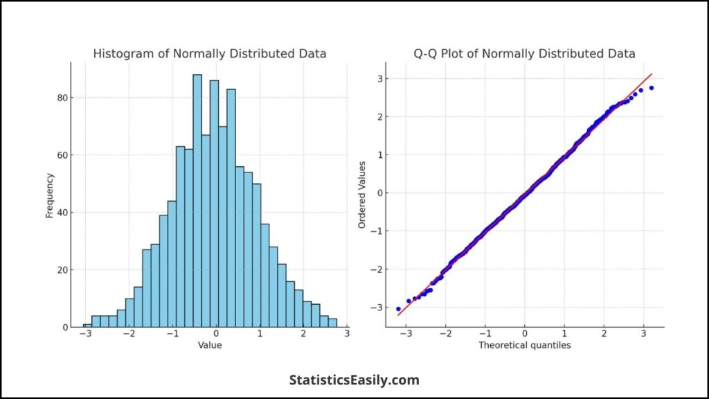
The paired samples t-test assumes that the differences between paired observations are normally distributed. This assumption does not necessitate the normality of the individual distributions of the two groups but rather the distribution of their differences. We can use the Shapiro-Wilk test to check the data adjustment for normality.

Visual Aid for Normality: A histogram or a Q-Q plot can be used to assess the normality of the differences. In a histogram, a bell-shaped curve suggests normality. The distribution can be considered normal in a Q-Q plot if the points roughly follow the line.

Addressing Violations:

Non-normal Distribution: If the differences between pairs do not follow a normal distribution, consider normalizing the data using transformations. A non-parametric alternative, such as the Wilcoxon signed-rank test, may be more appropriate if transformations are ineffective.

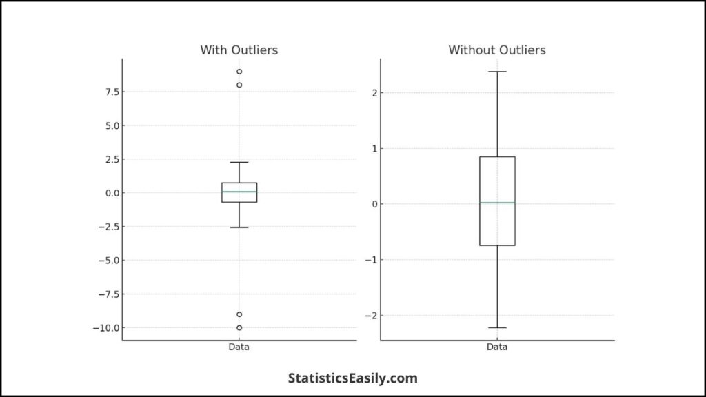
Outliers: Outliers can disproportionately affect the paired t-test, potentially leading to misleading results.

• Visual Aid for Outliers: Boxplots are particularly effective for identifying outliers. Points that fall outside the whiskers of the boxplot may be considered outliers.
• Handling Outliers: Investigate outliers for data entry errors or measurement anomalies once identified. If outliers are legitimate observations, consider their impact on the analysis carefully. In some cases, robust statistical techniques or adjustments may be necessary to mitigate their influence.

Practical Considerations

Conducting preliminary analyses to verify these assumptions before proceeding with the paired t-test is essential. This preemptive approach bolsters the validity of your findings and aligns with the principles of rigorous and ethical scientific inquiry.

---

Paired T-Test Procedure and Calculation

This section provides a detailed, step-by-step guide to performing a paired t-test, focusing on calculating mean differences, standard deviations, and the t-statistic, complemented by visual examples for clarity.

Data Collection and Preparation

1. Gather Data: Collect paired data from two sets of related measurements, ensuring each ‘before’ measurement is paired with its corresponding ‘after’ measurement. This could involve pre- and post-intervention assessments on the same subjects.
2. Clean Data: Verify that the data is clean, correctly matched, and free from outliers that could skew the results. Data cleaning is crucial for the accuracy of the test results.

Execution in R

1. Input Data: Import your data into R, arranging it into two columns representing the ‘before’ and ‘after’ conditions. Ensure each row corresponds to a matched pair.
2. Run Paired T-Test: Use R’s ‘t.test()’ function to perform the paired t-test. The basic syntax is ‘t.test(before, after, paired = TRUE)’, where ‘before’ and ‘after’ represent your data vectors. This function computes the t-statistic, p-value, and confidence interval for the mean difference.

# R code example
before <- c(1, 2, 3, 4, 5)  # Sample 'before' data
after <- c(2, 3, 4, 5, 6)   # Sample 'after' data

# Perform paired t-test
test_result <- t.test(before, after, paired = TRUE)

# Print the test result
print(test_result)

# Calculate Cohen's d for effect size
install.packages("effsize") # Install the effsize package if not already installed

library(effsize) # Run the effsize package

# Calculate the effect size
effect_size <- cohen.d(before, after, paired = TRUE)

# Output the effect size
print(effect_size)

Paired T-Test Calculation Details

Mean Difference: Calculate the difference between each pair of observations. The mean of these differences (D) is a crucial component of the t-test.

Standard Deviation of Differences: Compute the standard deviation of the differences (SD) to measure the dispersion.

T-Statistic: The t-statistic is calculated using the formula:

t = D / (SD / √n​)

where n is the number of pairs. This statistic measures how many standard deviations the mean difference is away from zero.

After calculating the t-statistic in a paired t-test, the subsequent steps involve determining the p-value and considering the degrees of freedom (df) to accurately interpret the test’s results. Here’s how to proceed:

Determining the P-Value

The p-value is a crucial component in hypothesis testing, indicating the probability of obtaining test results at least as extreme as the observed results, assuming the null hypothesis is true. After calculating the t-statistic:

1. Degrees of Freedom (df): For a paired t-test, the degrees of freedom are calculated as df = n−1, where n is the number of pairs. The degrees of freedom account for the number of values that are free to vary in the final calculation of a statistic.
2. Refer to the T-Distribution Table: With the calculated t-statistic and degrees of freedom, refer to a t-distribution table to find the p-value. The t-distribution table provides critical values for different degrees of freedom at various significance levels (alpha levels).
3. Software Computation: Statistical software like R automatically computes the p-value when conducting a t-test. The software uses the t-statistic and degrees of freedom to calculate the probability.

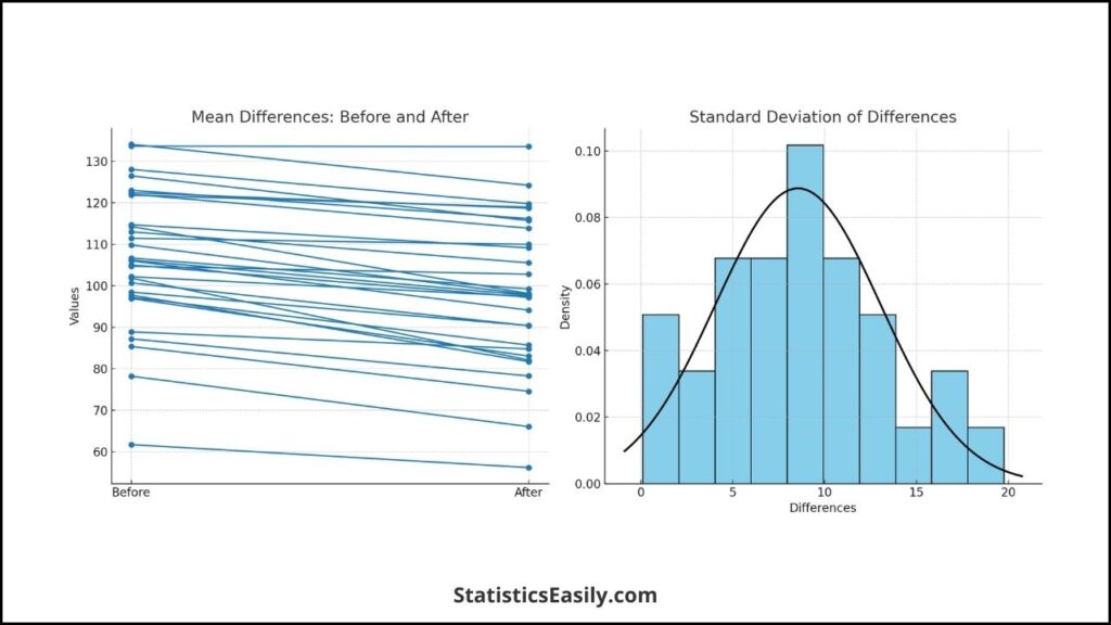
Visual Examples

Mean Differences: A line graph displaying each pair’s ‘before’ and ‘after’ values can visually represent the mean difference, highlighting the intervention’s effect.

Standard Deviation: A histogram of the differences with a superimposed normal curve can help visualize the differences’ spread and normality.

Interpretation of Results

1. P-Value: A p-value less than the alpha level (commonly set at 0.05) indicates a statistically significant difference between the paired groups, suggesting that the observed changes are unlikely to have occurred by chance.
2. Effect Size: Calculating the effect size, such as Cohen’s d, provides insight into the magnitude of the observed difference, adding context to the statistical significance.
3. Confidence Interval: The confidence interval for the mean difference offers a range within which the true mean difference is likely to lie, measuring the result’s precision.

---

Conclusion

In this comprehensive guide, we delved into the intricacies of the paired samples t-test. This statistical method plays a pivotal role in scientific research. This test is instrumental in comparing two sets of observations from the same subjects under different conditions, thereby providing a robust framework for evaluating the efficacy of interventions across various fields such as medicine, psychology, and education.

Key Points Summarized:

• The paired t-test enhances the precision of data analysis by controlling for individual variability, making it a powerful tool for discerning the true impact of treatments or interventions.
• Adherence to the test’s assumptions, including the normal distribution of paired differences and the independence of observations, is paramount for the validity of its outcomes.
• The paired t-test‘s practical applications span diverse disciplines, demonstrating its versatility and critical role in empirical research.
• Navigating potential pitfalls, such as mismatched pairs or overlooking outliers, requires meticulous data preparation and ethical statistical practices.

Reflecting on the broader context of scientific discovery, the paired t-test exemplifies the scientific method’s rigor, offering a window into the empirical truths that underpin our understanding of the natural world. Through careful execution and interpretation, the paired samples t-test contributes to the advancement of knowledge and upholds the principles of scientific integrity.

In essence, the paired t-test is more than a mere statistical tool; it is a testament to the enduring quest for knowledge. It embodies the scientific spirit, weaving together data threads into coherent narratives illuminating interventions’ efficacy and their impact on human well-being. As we harness the power of this analytical tool, we are reminded of the broader implications of our findings, not just for the academic community but for society at large.

In the grand tapestry of scientific inquiry, the paired t-test is a crucial stitch, binding empirical evidence with the philosophical ideals of truth. Through this synthesis, we can truly appreciate the contributions of statistical methods like the paired t-test to the enriching tapestry of human knowledge, driving forward the noble endeavor of scientific exploration for the betterment of all.

---

Recommended Articles

Explore more insights on statistical tests and data analysis by diving into our collection of related articles on the blog.

1. What is the Difference Between T-test vs. ANOVA
2. What is the Difference Between T-Test vs. Chi-Square Test?
3. What is the difference between t-test and Mann-Whitney test?

---

Frequently Asked Questions (FAQs)

Q1: What is a paired t-test used for? A paired t-test is primarily used to compare the means of two related groups to determine if there is a statistically significant difference between them. This test is ideal for ‘before and after’ studies or when measuring the same subjects under two conditions.

Q2: What is the difference between a paired t-test and ANOVA? While a paired t-test compares the means of two related groups, ANOVA (Analysis of Variance) is used when comparing the means of three or more groups or different levels of a factor. ANOVA can handle more complex designs than a simple paired comparison.

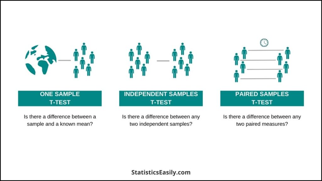
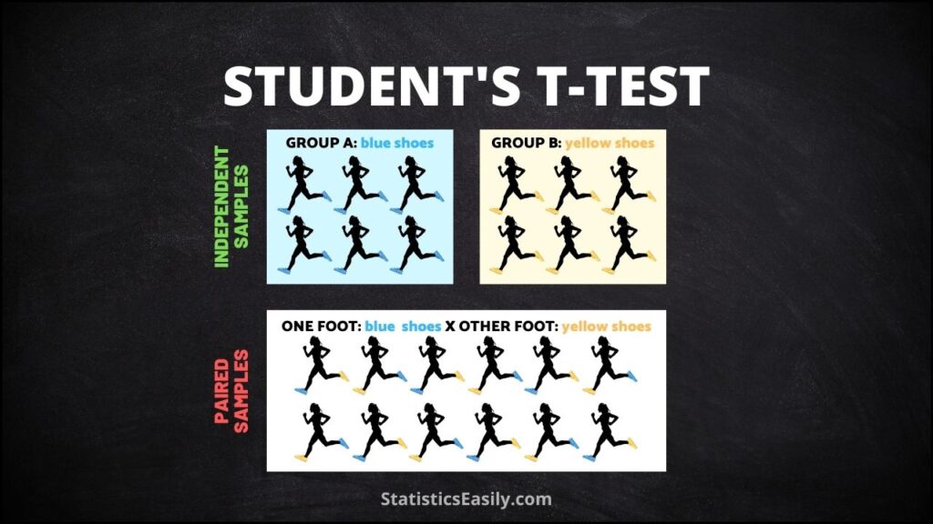
Q3: What are the 3 types of t-tests? The three main types of t-tests are: 1) One-sample t-test, comparing the mean of a single group against a known mean. 2) Independent two-sample t-test, comparing the means of two independent groups. 3) Paired t-test, comparing the means of the same group or matched subjects at two different times or under two different conditions.

Q4: What is the difference between a paired t-test and a one-sample t-test? A paired t-test compares the means of the same or matched subjects under two different conditions, focusing on the difference between these paired observations. In contrast, a one-sample t-test compares the mean of a single sample to a known or hypothesized population mean.

Q5: How do you perform a Paired T-Test in R? First, to conduct a paired t-test in R, ensure your data is structured with paired observations, typically in two columns where each row represents a pair. Using the ‘t.test()’ function, specify your two data vectors, and set the ‘paired’ argument to ‘TRUE’. The function will return the t-statistic, degrees of freedom, and p-value, among other information. Here’s a basic example, assuming ‘before’ and ‘after’ are your vectors of paired observations: ‘t.test(before, after, paired = TRUE)’. This command performs the paired t-test on your data, comparing the ‘before’ and ‘after’ conditions, and provides the statistical output necessary for interpretation.

Q6: Can a paired t-test be used for non-normal data? For significantly non-normal data, non-parametric alternatives like the Wilcoxon signed-rank test are recommended, as the paired t-test assumes normally distributed differences between pairs.

Q7: How do you interpret paired t-test results? Interpretation focuses on the p-value; if it’s below your chosen significance level (commonly 0.05), the difference between the paired groups is considered statistically significant, indicating a real effect beyond random chance.

Q8: What’s the difference between a paired t-test and an independent t-test? A paired t-test is used for related samples or matched pairs, analyzing the difference within pairs. An independent t-test compares the means of two independent or unrelated groups, focusing on the variance between the groups.

Q9: How does a paired t-test handle missing data? In a paired t-test, if one value in a pair is missing, the entire pair is typically excluded from the analysis. This approach prevents biases that might arise from imputing missing values. However, it can reduce the power of the test if many pairs are excluded.

Q10: Can a paired t-test be used for over two-time points? A paired t-test is designed for comparisons between two-time points or conditions. Repeated measures ANOVA or a mixed-effects model would be more appropriate for analyses involving more than two-time points to accommodate the additional complexity.