Sample Size in Logistic Regression: A Simple Binary Approach


This article will guide you through calculating the sample size for a Simple Binary Logistic Regression.
We will utilize the popular and freely available software G*Power, which is one of the most used for this purpose.
We were inspired to create this article after realizing that many online tutorials for G*Power-based sample size calculations are inaccurate.
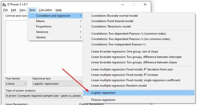
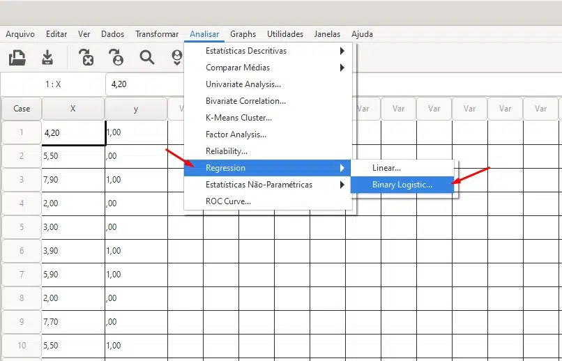
Upon downloading and installing G*Power, open it and choose the sample size calculation option for logistic regression analysis by clicking Tests: Correlation and regression: Logistic regression tab.
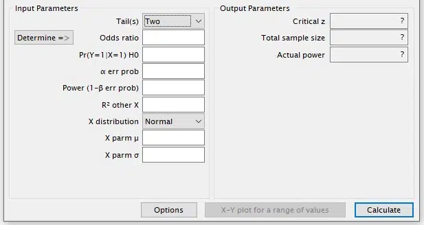
Next, input the following parameters:
In Tail(s), select One for one-tailed tests or Two for two-tailed tests.
A one-tailed test is appropriate for a specific alternative hypothesis, such as “increased value of X corresponds to a higher probability of the event occurring.“
A two-tailed test is suitable for a general alternative hypothesis, like “X influences event Y,” without an initial directional distinction.
Base your hypothesis on existing knowledge in your field. If unsure, opt for Two (two-tailed).
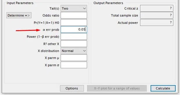
The significance level (α) represents the probability of rejecting the null hypothesis when it is true, leading to a type I error.
Typically, α is set at 0.05 or 0.01. An α of 0.05, for instance, indicates a 5% risk of concluding a significant relationship exists when none actually does.
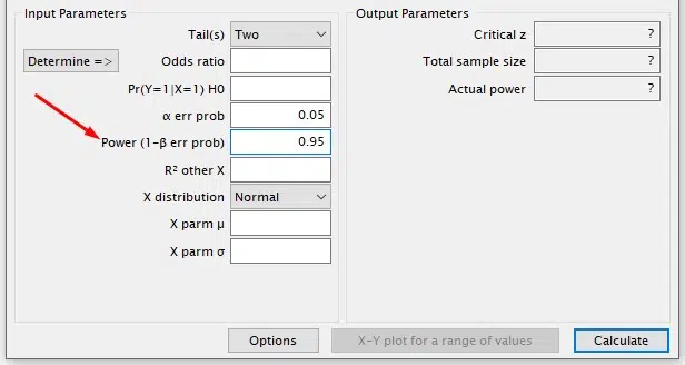
The Test Power (1 – β) is the probability of rejecting the null hypothesis if false, effectively controlling for type II error (β).
Acceptable values usually range from 0.80 to 0.99. Higher test power is preferable but also increases the required sample size.
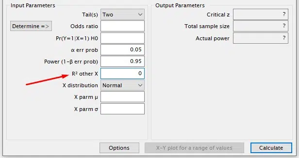
Since simple binary logistic regression models only have one independent variable, set this value to zero.
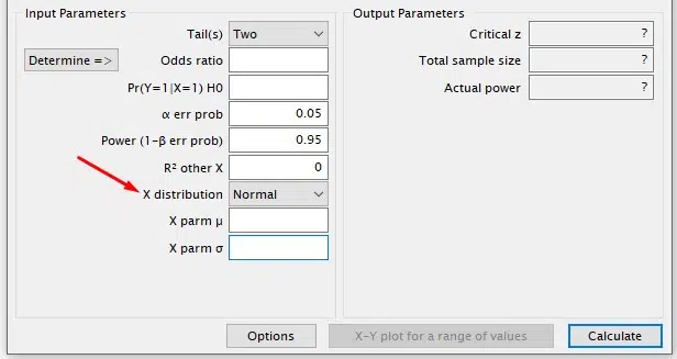
Select the distribution type for variable X, which is the independent or predictor variable in the model.
Choose Binomial for binary variables, Normal for continuous quantitative variables, and Poisson for discrete variables. Use other available distributions only if necessary.
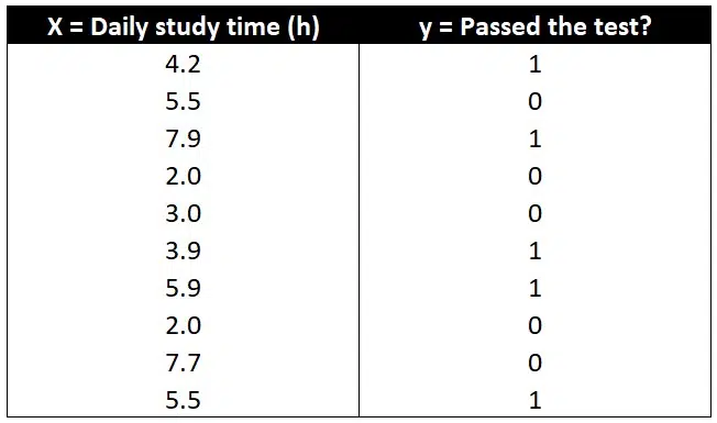
The last four parameters require population estimates from a pilot study, similar research, or theoretical calculations.
If possible, use data from a pilot study, as we will demonstrate here.
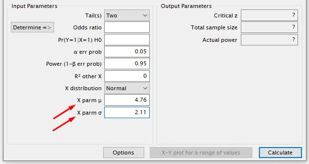
Enter variable X’s mean and standard deviation from the pilot study data for the Population Mean of Variable X and Population Standard Deviation of Variable X parameters, respectively.
Obtain the final two parameters through a preliminary simple logistic regression analysis with the pilot study data.
For our demonstration, we will use the free and easy-to-use PSPP software. Any software capable of running logistic regression can be used.
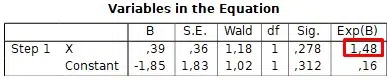
The odds ratio indicates the association between an exposure and an outcome and measures effect size.
Perform a preliminary analysis with the pilot data in PSPP to obtain the odds ratio value (Exp(B) for variable X, 1.48 in this example) and enter it in G*Power.
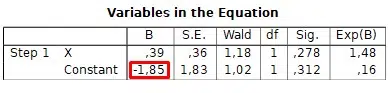
The final parameter is the probability of occurrence of the dependent variable (y = 1) when the null hypothesis (H0) is true, i.e., when the coefficient of the independent variable (X) equals 0, and the model only contains the intercept.
To calculate this value, enter the constant (intercept) estimate B from the previous step into the following Excel formula:
=EXP(B)/(1+EXP(B))
For our example:
=EXP(-1.85)/(1+EXP(-1.85))
=0.1355
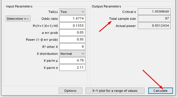
With all parameters entered in G*Power, click Calculate to obtain the sample size determined by the calculation!
In our example, the sample size required to identify the estimated odds ratio is 97 individuals randomly sampled from the target population.
By following these steps and using G*Power, you can effectively calculate the appropriate sample size for a Simple Binary Logistic Regression analysis.
This process allows you to optimize your study design, minimize errors, and improve the validity of your findings.
Furthermore, understanding the role of different parameters in determining sample size contributes to a comprehensive grasp of logistic regression as a whole.
Want to learn how to calculate sample size in G*Power for the most crucial inferential analyses?
Don’t miss out on the FREE samples of our recently launched digital book!
Inside, you’ll master sample size calculation for independent or paired t-tests; one- or two-way ANOVA, with or without repeated measures, and mixed models; simple and multiple linear and logistic regression, and more.
Click this link and discover everything it has to offer: Applied Statistics: Data Analysis.

Dive deep into the foundations of data analysis, exploring the four fundamental levels of measurement: nominal, ordinal, interval, and ratio scales.

Explore the distinctions between incidence vs. prevalence to enhance your understanding of epidemiological studies and public health.

Sample Size T-Test: Improve the reliability of your t-test results with our step-by-step guide on calculating the ideal sample size.

This comprehensive guide explores how Principal Component Analysis transforms complex data into insightful, truthful information.

Discover how to select the perfect graph for your data. Learn about quantitative and qualitative variables and explore different graph types.

Master One Way ANOVA with this guide, covering assumptions, effect sizes, post hoc tests, common mistakes, and best practices.