Principal Component Analysis: Transforming Data into Truthful Insights

You will learn the power of Principal Component Analysis in revealing hidden data truths.

---

Introduction

Principal Component Analysis (PCA) is a crucial technique in statistics and data science, offering a sophisticated method for reducing the dimensionality of large data sets while preserving as much of the data’s variability as possible. This process simplifies the complexity inherent in multidimensional data. It enhances the interpretability without significantly compromising the integrity of the original data. At its core, PCA seeks to identify patterns in data, spotlight discrepancies, and transform complex datasets into a more straightforward form, enabling analysts and scientists to uncover meaningful insights more efficiently. This article aims to demystify PCA, guiding readers through its conceptual foundations, practical applications, and the profound impact it can have on data analysis strategies. By focusing on PCA, we aim to illuminate the path for enthusiasts and professionals, fostering a deeper understanding and mastery of this indispensable analytical tool.

---

Highlights

• PCA reduces data dimensions while preserving data’s essential characteristics.
• Historically, PCA has evolved from simple concepts to complex applications in genomics and finance.
• Using PCA correctly can unveil patterns in data that were not initially apparent.
• Choosing the correct number of components in PCA is crucial for accurate data interpretation.
• PCA tools and software streamline the analysis, making data insights more accessible.

---

The Essence of Principal Component Analysis

Principal Component Analysis (PCA) is a statistical procedure that uses an orthogonal transformation to convert a set of observations of possibly correlated variables into values of linearly uncorrelated variables called principal components. This technique is widely recognized for its ability to reduce the dimensionality of data while retaining most of the variation in the dataset. The essence of PCA lies in its ability to extract the essential information from the data table, compress the size of the data set, and simplify the description of the data set while preserving the most valuable parts of all of the variables.

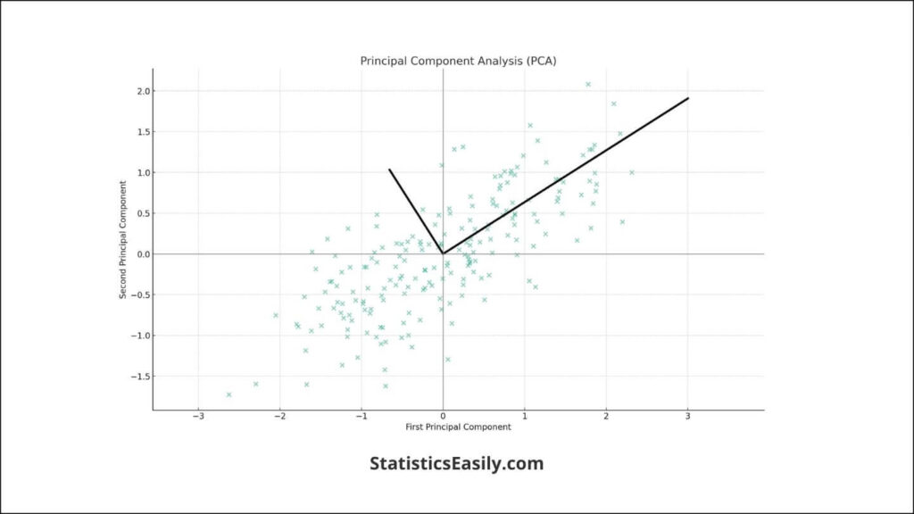
The core principles of PCA involve identifying directions, or axes, along which the variability in the data is maximized. The first principal component is the direction that maximizes the variance of the data. The second principal component is orthogonal to the first. It identifies the direction of the following highest variance, and so on. This process allows PCA to reduce complex data sets to a lower dimension, making it easier to analyze and visualize the data without significant loss of information.

PCA’s beauty in simplifying complex data sets while retaining essential information is unparalleled. It enables data scientists and statisticians to uncover hidden patterns in the data, facilitating more informed decision-making. By focusing on the most significant components, PCA helps highlight the underlying structure of the data, thus providing a clearer insight into the true nature of the data being analyzed. This method enhances the efficiency of data analysis. It contributes to a more truthful and profound understanding of the data’s intrinsic properties.

---

Historical Background and Theoretical Foundations

The journey of Principal Component Analysis (PCA) traces back to the early 20th century, rooted in the pioneering work of Karl Pearson in 1901. Pearson, in his quest to understand the underlying data structure, developed PCA to describe the observed variability in a multidimensional data space through uncorrelated variables. This technique was later mathematically formalized by Harold Hotelling in the 1930s, providing a more robust statistical foundation and expanding its applicability across various scientific domains.

The mathematical foundations of PCA are deeply entwined with linear algebra, particularly the concepts of eigenvectors and eigenvalues. At its core, PCA transforms the original data into a new coordinate system where the most significant variances by any data projection lie on the first coordinates, known as principal components. This transformation is achieved through the eigendecomposition of the data covariance matrix or singular value decomposition (SVD) of the data matrix. These methods ensure variance maximization and preserve the dataset’s structural integrity.

The precision and truthfulness of PCA lie in its mathematical rigor. PCA encapsulates the data’s inherent variability and relationships between variables using the covariance matrix, offering a distilled view highlighting the most significant patterns. This process not only simplifies the complexity of data but also brings the essential truth — the underlying structure and variability of the data — to the forefront, allowing for insightful analysis and decision-making.

PCA has established itself as a cornerstone of statistical data analysis through its development and mathematical underpinnings. Its ability to reduce dimensionality while preserving essential information has made it an invaluable tool for data scientists and statisticians, facilitating a deeper understanding of data across numerous fields.

---

Practical Applications of Principal Component Analysis

Principal Component Analysis (PCA) has transcended its academic origins to become an essential analytical tool across multiple domains. Its capability to distill large datasets into manageable insights has revolutionized how we interpret complex information, making it invaluable in fields as diverse as genomics, finance, and digital image processing.

In genomics, PCA simplifies genetic data, often involving thousands of variables. By reducing dimensionality, PCA allows researchers to identify genetic markers and patterns related to diseases more efficiently, facilitating breakthroughs in personalized medicine and evolutionary studies.

The finance sector leverages PCA for risk management and investment strategies. PCA can highlight the principal factors affecting market variations by analyzing the covariance matrix of asset returns. This simplification aids in portfolio diversification, highlighting underlying trends that might not be apparent through traditional analysis.

In image compression, PCA reduces the redundancy in pixel data, enabling the efficient storage and transmission of images without significant loss of quality. This application is critical in fields where bandwidth is limited, such as satellite imagery and telemedicine, and it’s essential to balance compression with the retention of image integrity.

PCA reveals underlying patterns in data through these applications and significantly simplifies decision-making processes. By distilling complex datasets into their most meaningful components, PCA reflects the inherent goodness in data analysis — transforming overwhelming data volumes into actionable insights. This transition from complexity to clarity enhances our understanding of the data. It allows us to make informed decisions across a spectrum of critical fields, showcasing PCA’s versatility and enduring relevance.

---

Step-by-Step Guide to Performing Principal Component Analysis on Python

Performing Principal Component Analysis (PCA) in Python efficiently condenses large datasets into their most significant components, simplifying data analysis. This guide walks through the process from data preparation to interpretation, utilizing the scikit-learn library, renowned for its powerful data mining and analysis tools.

1. Data Preparation

Before implementing PCA, ensure your data is suitable for the process. This means handling missing values, normalizing the data, and reducing features if they are highly correlated.

import pandas as pd
from sklearn.preprocessing import StandardScaler

# Load dataset
df = pd.read_csv('data_pca.csv')

# Preprocessing
## Handle missing values if any
df.fillna(method='ffill', inplace=True)

## Feature scaling
features = ['Feature1', 'Feature2', 'Feature3', 'Feature4', 'Feature5', 'Feature6']
x = df.loc[:, features].values
x = StandardScaler().fit_transform(x)  # Normalize data

2. Implementing PCA

With the data prepared, you can apply PCA. Decide the number of principal components you wish to retain or let the algorithm choose based on variance.

from sklearn.decomposition import PCA

# PCA transformation
pca = PCA(n_components=2)  # n_components to specify desired reduction
principalComponents = pca.fit_transform(x)

# Convert to a DataFrame
principalDf = pd.DataFrame(data=principalComponents, columns=['Principal Component 1', 'Principal Component 2'])

3. Analyzing the Results

After transforming the data, analyze the principal components to understand the dataset’s underlying structure.

print(pca.explained_variance_ratio_)

This prints the variance explained by each of the selected principal components, which gives insight into how much information is captured by the analysis.

4. Visualization

Visualizing the principal components can provide intuitive insights into the data structure and clustering.

import matplotlib.pyplot as plt

plt.figure(figsize=(8,6))
plt.scatter(principalDf['Principal Component 1'], principalDf['Principal Component 2'])
plt.xlabel('Principal Component 1')
plt.ylabel('Principal Component 2')
plt.title('PCA on Dataset')
plt.show()

5. Interpretation

Interpretation involves understanding the principal components in terms of original features. This often requires domain knowledge and a look at the PCA components’ weights.

# Accessing the components_
print(abs(pca.components_))

This shows the weight of each original feature in the principal components, aiding in interpreting the components.

Example Dataset Results

Using a hypothetical dataset, the PCA might reveal that the first two principal components capture significant portion of the variance in the data. Visualization might show clear clustering, suggesting distinct groups within the dataset. The component weights could indicate which features most influence these groupings.

---

Step-by-Step Guide to Performing Principal Component Analysis on R

Performing Principal Component Analysis (PCA) in R efficiently condenses large datasets into their most significant components, simplifying data analysis. This guide walks through the process from data preparation to interpretation, utilizing the versatile and comprehensive set of tools available in R for statistical computation.

1. Data Preparation

Before implementing PCA, make sure your data is appropriate for the process. This involves handling missing values, standardizing the data, and reducing features if they are highly correlated.

# Load dataset
df <- read.csv('data_pca.csv')

# Preprocessing
## Handle missing values if any
df[is.na(df)] <- method = na.omit(df)

## Feature scaling
features <- df[, c('Feature1', 'Feature2', 'Feature3', 'Feature4', 'Feature5', 'Feature6')]
scaled_features <- scale(features) # Normalize data

2. Implementing PCA

With the data prepared, PCA can be applied. You can decide the number of principal components you wish to retain or let the algorithm choose based on explained variance.

# PCA transformation
pca <- prcomp(scaled_features, rank. = 2, center = TRUE, scale. = TRUE)

# The rank. argument specifies the desired reduction
# prcomp automatically centers and scales the variables

3. Analyzing the Results

After transforming the data, the summary of the PCA object can be used to understand the variance explained by the principal components.

# This prints the summary of the PCA object
summary(pca)

4. Visualization

Visualizing the principal components can offer intuitive insights into the data structure and possible clustering.

# This creates a scatter plot of the first two principal components
plot(pca$x[, 1:2], col = df$YourGroupVariable, xlab = 'Principal Component 1', ylab = 'Principal Component 2', main = 'PCA on Dataset')

5. Interpretation

Interpreting PCA involves understanding how the original features contribute to the principal components, often requiring domain knowledge.

# This shows the loading of each original feature on the principal components
pca$rotation

Example Dataset Results

Using a hypothetical dataset, PCA in R might reveal that the first two principal components capture a significant portion of the variance in the data. Visualization might show apparent clustering, suggesting distinct groups within the dataset. Examining the rotation (loadings) can indicate which features most influence these groupings.

---

Best Practices and Common Pitfalls

Adhering to best practices and remaining vigilant of common pitfalls is crucial to interpreting meaningful data through principal component analysis (PCA). Accuracy and the true representation of the dataset’s essence are essential.

Ensuring Accuracy

• Data Standardization: Always standardize your data before applying PCA, as the analysis is sensitive to the variances of the initial variables.
• Missing Values: Address any missing or infinite values in the dataset to prevent biases in the component extraction.
• Outliers: Investigate and understand outliers before PCA, as they can disproportionately influence the results.

Avoiding Misinterpretations

• Component Interpretability: The principal components are mathematical constructs that may not always have a direct real-world interpretation. Take care not to overinterpret them.
• Variances: A high variance ratio for the first few components doesn’t guarantee that they hold all the meaningful information. Important subtleties may exist in components with lower variance.

Choosing the Correct Number of Components

• Explained Variance: Use a scree plot or cumulative explained variance ratio to identify an elbow point or the number of components that capture substantial information.
• Parsimony: Balance complexity with interpretability, selecting the smallest number of components that still provide a comprehensive view of the data structure.
• Domain Knowledge: Leverage understanding from your field to decide how many components to retain, ensuring they make sense for your specific context.

Staying True to Data’s Essence

• Consistency with Objectives: Align the number of components retained with the analytic goals, whether data simplification, noise reduction, or uncovering latent structures.
• Comprehensive Review: Combine PCA with other data exploration techniques to build a holistic understanding of the data.

Following these guidelines will steer your PCA toward a reliable analysis, preserving the integrity of the data while extracting actionable insights. By remaining cautious of the intricacies involved in PCA, one can avoid the pitfalls that lead to misinterpretation and ensure that the analysis remains an authentic reflection of the underlying dataset.

---

Advanced Topics in Principal Component Analysis

As the data landscape continues to expand and diversify, Principal Component Analysis (PCA) evolves, embracing its classic roots and innovative expansions to address the complexity of modern data structures. This journey into PCA’s advanced topics reveals the method’s versatility and enduring adaptability in data science.

Variations of PCA

• Kernel PCA: This extension of PCA is used for nonlinear dimensionality reduction. Using kernel methods effectively captures the structure in data where the relationship between variables is not linear, thus uncovering patterns that traditional PCA might miss.
• Sparse PCA: In datasets where features outnumber observations, Sparse PCA shines by producing principal components with sparse loadings. This results in a more interpretable model, highlighting a smaller subset of features, which is particularly useful in high-dimensional data scenarios like genomics.

Extensions of PCA

• Incremental PCA: For massive datasets that cannot fit in memory, Incremental PCA offers a solution. It breaks down the PCA computation into manageable mini-batches, updating the components incrementally, which is also advantageous for streaming data.
• Robust PCA: Outliers can significantly affect the outcome of PCA. Robust PCA mitigates this by separating the sparse outliers from the low-rank structure, ensuring that anomalous points do not skew the core data.

---

Conclusion

Principal Component Analysis (PCA) has been firmly established as an indispensable technique in the data analysis toolbox. It facilitates a deeper understanding of data by extracting its most informative elements. This guide has sought to clarify PCA’s methodology, from its foundational mathematics to its application across various fields. We’ve underscored its utility in reducing dimensionality while preserving data’s inherent structure. This process aids significantly in both visualization and subsequent analyses. Researchers and data scientists are encouraged to integrate PCA into their workflows to enhance the interpretability of complex datasets. When implemented thoughtfully, PCA yields insights into the dominant patterns within data and streamlines the path toward more robust and informed decision-making.

---

Recommended Articles

Explore our blog’s rich library of articles on related topics to discover more about data analysis.

1. Richard Feynman Technique: A Pathway to Learning Anything in Data Analysis
2. Understanding Distributions of Generalized Linear Models
3. Can Standard Deviations Be Negative? (Story)
4. Box Plot: A Powerful Data Visualization Tool
5. Generalized Linear Models (Story)

---

Frequently Asked Questions (FAQs)