

Data Structures: A Data Scientist’s Guide
This post helps data practitioners understand fundamental data structures to write faster, more memory-efficient code.
A common bottleneck in data processing scripts, from sluggish feature engineering loops to inefficient lookups, can often be traced to a mismatch between the task and the underlying data structure being used. The root cause of these performance pain points often lies not in the logic of your code, but in how that data is organized in memory. Understanding these structures—and their trade-offs—is a fundamental skill for writing efficient and scalable analysis pipelines. This post will distill key lessons on data structures from Harvard’s renowned CS50x course, connecting these computer science fundamentals directly to the practical world of data analysis and data science. Este post é uma síntese baseada no CS50x 2025 (Harvard) no YouTube.
1. Arrays and Their Hidden Resizing Cost
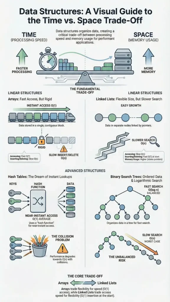
An array is a simple data structure where elements of the same type are stored back-to-back (“contiguous”) in memory. This contiguous layout makes accessing any element by its index extremely fast. However, arrays come with a critical limitation: you must decide their size in advance.
What happens when you need to “grow” an array that’s already full? You can’t simply add a new element at the end if that memory location is already occupied. The only solution is to allocate a completely new, larger block of memory, manually copy every single element from the old array to the new one, and then free the memory used by the original array. This process of copying is a time-consuming, “linear time” operation—the bigger the array, the longer it takes.
Data Science Connection
Many common data tools, like Python lists, behave like “dynamic arrays.” While they seem to grow automatically, they perform this costly resizing under the hood. To make appends fast, Python lists use over-allocation—reserving extra space—which results in amortized constant time (amortized O(1)) for appends. However, inserting an item at the beginning of a large list is slow not just because of potential resizing, but because it requires shifting every subsequent element one position to the right, a direct O(n) cost.
2. Linked Lists: Trading Contiguous Memory for Flexibility
A linked list offers a solution to the array’s rigid resizing problem. Instead of storing elements contiguously, a linked list is a series of “nodes” that can be located anywhere in memory. Each node contains two things: a piece of data and a “pointer” (an address) that links to the location of the next node. This allows you to “stitch together” available memory locations as needed.
This structure introduces a primary trade-off:
- Upside: The list can grow and shrink dynamically without the need to move all existing elements. This makes more efficient use of fragmented memory.
- Downside: It uses more memory overall, because every single element requires an extra pointer to store the address of the next one.
- Critical Downside: You lose the ability to perform a fast binary search. Because elements are not stored contiguously, you cannot instantly jump to the middle of the list; you must traverse it one node at a time from the very beginning.
Data Science Connection
Consider a real-time event log where events might need to be inserted or removed from the middle of a sequence based on updates. A standard Python list would be punishingly slow for this, as each operation could require shifting many elements. A structure like Python’s collections.deque, however, is implemented using a doubly-linked list, providing fast O(1) appends and pops from both ends.
3. The Counter-Intuitive Truth: The Fastest List is Built Backwards
When working with a linked list, how you add new elements has a dramatic impact on performance. To add a new node to the beginning of the list (prepending), you only need to create the new node and update a couple of pointers at the head of the list. This operation is independent of the list’s total size.
This makes prepending a constant time (O(1)) operation—it’s incredibly fast. In contrast, to add a new node to the end of the list (appending), you must first traverse the entire list from the beginning to find the final node. This makes appending a linear time (O(n)) operation, which gets progressively slower as the list grows.
The surprising result is that the most performant way to build a linked list from scratch is to add each new element to the front. This means if you insert the numbers 1, then 2, then 3, the final list in memory will read 3 -> 2 -> 1.
Data Science Connection
This is a classic example of how a seemingly simple choice—adding to the front versus the back—can have massive performance implications (O(1) vs. O(n)). This highlights the importance of understanding the time complexity of the operations we use daily in data cleaning and feature engineering scripts. A slow-running loop might be hiding a linear-time operation that could be optimized.
4. Binary Search Trees: Fast Searches That Can Degenerate
A binary search tree (BST) attempts to combine the best of both worlds: the fast search capability of a sorted array and the dynamic resizing of a linked list. It’s a tree of nodes where each node has up to two children. The structure is governed by the “binary search property”: for any given node, all values in its left subtree are smaller, and all values in its right subtree are larger.
This property allows for a binary search by simply following left or right pointers down the tree, achieving an efficient logarithmic time (O(log n)) search performance on average. However, the BST has a critical flaw. In the “perverse case” where you insert data that is already sorted (e.g., inserting 1, then 2, then 3, then 4), the tree becomes completely unbalanced. Each new node is simply added to the right of the previous one.
In this worst-case scenario, the binary search tree “devolves into a linked list.” Its search performance degrades from logarithmic time to slow, linear time (O(n)).
Data Science Connection
The unbalanced BST is a powerful metaphor for the difference between average-case and worst-case performance. In data science, the distribution and order of our input data can dramatically affect an algorithm’s efficiency. This is why database indexes, which are often based on tree structures, require complex “balancing” algorithms to continuously reorganize themselves and prevent this worst-case scenario from occurring.
5. Hash Tables: The Practical Path to Constant Time
The hash table is the go-to data structure for implementing dictionaries, which store key-value pairs. It masterfully combines arrays and linked lists to achieve near-instant lookups. Its core components are:
- An array of “buckets.”
- A hash function that takes a key (e.g., a person’s name) and deterministically converts it into an index for the array.
- Linked lists within each bucket to handle “collisions”—the cases where two different keys hash to the same array index.
The lecture’s analogy of Sweetgreen’s pickup shelves perfectly illustrates this. Your name on the order is the key. The employee looking at the first letter of your name to choose a shelf (A-E, F-J, etc.) is the hash function. The shelf itself is the bucket (an index in the array). The few salads on that shelf you have to scan through represent the linked list for handling collisions. While the theoretical worst case is linear time (O(n)) if all keys collide into one long linked list, the practical, average-case performance is remarkably close to constant time (O(1)).
“yes, hash tables technically are in N divided by K which is really just Big O of n but in practice if you are smart and if you are clever about the hash function you use… the probability of collisions is probably going to be so low that even if occasionally the thing devolves into linear time most of the time it’s going to be indeed constant time aka Big O of one.” — Harvard CS50x 2025 (YouTube) — Lecture: Data Structures
Data Science Connection
Hash tables are the engine behind Python’s dictionaries (dict) and sets (set). This is why key lookups (my_dict['key']) and membership testing (item in my_set) are exceptionally fast. These structures are fundamental tools for performant data manipulation, creating lookup tables, aggregating data by category, and building features efficiently.
What to Apply Today
- Always prefer a dictionary/hash map for key-value lookups over searching through a list of pairs. The performance difference between O(1) and O(n) is enormous on large datasets.
- Be mindful of data order when performance matters. As seen with binary search trees, inserting sorted data into certain structures can trigger worst-case behavior.
- Question if your data needs to be ordered. If you only need fast lookups and membership tests, a set (hash-based) is far more efficient than a list.
- Visualize the underlying operations. When a script is slow, think about whether you are forcing a linear O(n) operation inside a loop, inadvertently creating O(n²) complexity.
- Recognize the time-space trade-off. A hash table (like a Python
dict) consumes more memory than a list to store its hash values and pointers, but it buys you dramatically faster lookups—a trade-off that is essential to writing performant code.
Closing
The central theme is that every data structure represents a trade-off between time, space, and implementation complexity. There is no single “best” structure, only the most appropriate one for the task at hand. The lecture transitions next to Python, a language that abstracts away many of the manual memory management details we’ve discussed. However, the performance principles remain just as critical, as these structures are still operating under the hood. Which data structure that you use every day will you now think about differently?