Kruskal-Wallis Test: Mastering Non-Parametric Analysis for Multiple Groups

You will learn the essential steps to accurately applying the Kruskal-Wallis Test in diverse research scenarios.

---

Introduction

Imagine understanding how different medications impact patient recovery times without assuming a normal data distribution. Enter the Kruskal-Wallis Test, a powerful tool in non-parametric statistical analysis that transcends the limitations of traditional parametric tests. Designed for comparing median values across multiple groups, this test is important for researchers dealing with non-normal or ordinal data distributions. It provides:

• A robust method for discerning significant differences;
• Ensuring that insights gleaned from diverse datasets are both accurate and reliable;
• Marking a pivotal advancement in statistical methodologies.

---

Highlights

• The Kruskal-Wallis Test is ideal for non-normal data distribution.
• It compares medians across multiple groups effectively.
• There is no need for data to meet strict variance homogeneity.
• Applicable for both small and large sample sizes.
• Interpreting H statistics and p-values reveals group differences.

---

Background and Theory

In statistical analysis, non-parametric statistics provide a vital framework for analyzing data without relying on the traditional assumptions of parametric tests, such as normal distribution or homogeneity of variances. Non-parametric methods, including the Kruskal-Wallis Test, are particularly useful for handling ordinal data or when the sample size is too small to validate the distribution assumptions required by parametric tests.

Understanding Non-Parametric Statistics

Non-parametric statistics do not presume an underlying probability distribution for the analyzed data. This makes them highly versatile and applicable in various situations where parametric assumptions cannot be met. Non-parametric tests are particularly useful for skewed distributions and ordinal data, offering a robust alternative when the data’s measurement scale does not support parametric assumptions.

The Kruskal-Wallis Test: A Closer Look

The Kruskal-Wallis Test is a non-parametric alternative to the one-way ANOVA and is used to determine if there are statistically significant differences between two or more groups of an independent variable on a continuous or ordinal dependent variable. It’s particularly noteworthy for its application across multiple groups where the assumptions of ANOVA are not tenable.

Assumptions

• The dependent variable should be continuous, ordinal, or count data.
• The dependent variable should be continuous or ordinal.
• The independent variable should consist of two or more categorical, independent groups.
• Observations across groups should be independent.

Note: The data does not need to follow a normal distribution, making the Kruskal-Wallis Test a non-parametric method.

Comparison with ANOVA

While the ANOVA test relies on the data meeting assumptions of normality and homogeneity of variances, the Kruskal-Wallis Test does not. Instead, it ranks the data and compares the sums of these ranks between groups, making it suitable for non-normal distributions and ordinal data. However, unlike ANOVA, it does not directly test for mean differences but rather for differences in the median or distribution between groups.

Key Takeaways

• Non-parametric statistics, like the Kruskal-Wallis Test, are essential when data do not meet the normality assumption.
• The Kruskal-Wallis Test is valuable for analyzing differences across multiple groups without the stringent assumptions required by parametric tests like ANOVA.
• It is applicable to a wide range of fields and research scenarios, making it a versatile tool in statistical analysis.

---

Effect Size and Types in the Kruskal-Wallis Test

The Kruskal-Wallis Test identifies significant differences across multiple groups, but discerning the practical impact of these differences necessitates the calculation of effect sizes. Effect size metrics translate statistical significance into quantifiable impact measures, crucial for real-world application and interpretation.

Standard Measures of Effect Size

Adapted Eta Squared (η²): Traditionally used in ANOVA, η² can be adapted for Kruskal-Wallis by relating the test’s H statistic to the total variance. This adaptation offers an estimate of the effect’s magnitude. However, it should be interpreted with the non-parametric nature of the data in mind.

Epsilon Squared (ε²): Designed for the Kruskal-Wallis Test, ε² provides insight into the variance explained by group differences, considering the non-parametric ranking of data. It’s a nuanced measure that complements the test’s findings by quantifying effect size without relying on parametric assumptions.

Additional Non-Parametric Effect Size Measures

Cohen’s d (Adapted for Non-Parametric Use): When conducting post-hoc pairwise comparisons, an adapted version of Cohen’s d can be applied to quantify the standardized difference between groups. This adaptation should account for the rank-based nature of the comparisons.

Rank-Biserial Correlation: This measure offers an intuitive effect size as a correlation coefficient by comparing mean ranks between groups. It’s particularly user-friendly, providing a straightforward interpretation of effect size that’s accessible to a broad audience.

Incorporating these effect size calculations into Kruskal-Wallis Test analyses enriches the statistical narrative, ensuring that findings are statistically significant and carry clear implications for practical application. By quantifying the magnitude of group differences, researchers can convey their results’ real-world relevance more effectively.

---

Post-Hoc Tests for Kruskal-Wallis Test

Upon finding significant results with the Kruskal-Wallis Test, it’s often necessary to perform post-hoc tests to pinpoint where the differences lie between groups. These tests provide:

• Detailed pairwise comparisons;
• Helping to understand which specific groups differ from each other;
• Thus offering more profound insights into the data.

After identifying significant results with the Kruskal-Wallis Test, post-hoc analyses are essential for pinpointing specific group differences. Here are the critical tests:

Dunn’s Test

• What it is: A widely-used non-parametric method for comparing ranks between pairs of groups.
• Usage: Preferred for detailed analysis after a Kruskal-Wallis Test indicates significant overall differences.
• Characteristics: Incorporates adjustments for multiple comparisons, minimizing the risk of Type I errors.

Nemenyi Test

• What it is: The Nemenyi Test is a non-parametric approach similar to the Tukey HSD test used in ANOVA, designed for conducting multiple pairwise comparisons based on rank sums.
• Usage: This test follows a significant Kruskal-Wallis Test, mainly when the objective is to compare every group against every other group.
• Characteristics: It offers a comprehensive analysis without assuming normal distributions, making it applicable to various data types. The test is beneficial for providing a detailed overview of the pairwise differences among groups.

Conover’s Test

• What it is: A non-parametric test for pairwise group comparisons, akin to Dunn’s Test, but employs a distinct method for p-value adjustment.
• Usage: Applied when a more nuanced pairwise comparison is desired post-Kruskal-Wallis.
• Characteristics: Provides an alternative p-value adjustment method suitable for various data types.

Dwass-Steel-Critchlow-Fligner (DSCF) Test

• What it is: A non-parametric method tailored for multiple pairwise comparisons.
• Usage: Ideal for post-Kruskal-Wallis analysis, offering a comprehensive pairwise comparison framework without normal distribution assumptions.
• Characteristics: Adjusts for multiple testing, ensuring the integrity of statistical conclusions.

Mann-Whitney U Test

• What it is: Also known as the Wilcoxon rank-sum test, it compares two independent groups.
• Usage: Suitable for pairwise comparisons post-Kruskal-Wallis, especially when analyzing specific group differences.
• Considerations: Not designed for multiple comparisons; adjustments (like the Bonferroni correction) are necessary to manage the Type I error rate.

Each test has unique features and applicability, making them valuable tools for post-hoc analysis following a Kruskal-Wallis Test. The specific research questions, data characteristics, and the need for Type I error control should guide the choice of test.

---

When to Use the Kruskal-Wallis Test

The Kruskal-Wallis Test is a non-parametric method for comparing medians across multiple independent groups. It is beneficial in scenarios where the assumptions required for parametric tests like ANOVA are violated. Below are specific situations where the Kruskal-Wallis Test is most appropriate:

Non-Normal Data Distributions: When the data does not follow a normal distribution, especially with small sample sizes where the Central Limit Theorem does not apply, the Kruskal-Wallis Test provides a reliable alternative.

Ordinal Data: This test can compare groups effectively for data measured on an ordinal scale, where numerical differences between levels are not consistent or meaningful.

Heterogeneous Variances: In cases where the groups have different variances, the Kruskal-Wallis Test can still be applied, unlike many parametric tests that require homogeneity of variances.

Small Sample Sizes: When sample sizes are too small to check the assumptions of parametric tests reliably, the Kruskal-Wallis Test can be a more suitable choice.

Examples:

By applying the Kruskal-Wallis Test in these scenarios, researchers can obtain reliable insights into group differences without the stringent assumptions required by parametric tests. This enhances the robustness and applicability of statistical analyses across diverse research fields, ensuring findings are grounded in accurate, methodologically sound practices.

Clinical Research: Comparing the effect of three different medications on pain relief, where pain relief levels are rated on an ordinal scale (e.g., no relief, mild relief, moderate relief, complete relief).

Environmental Science: Assessing the impact of various pollutants on plant growth where the growth is categorized into ordinal levels (e.g., no growth, slow growth, moderate growth, high growth), and the data is skewed or does not meet normality assumptions.

Marketing Studies: Evaluating customer satisfaction across multiple stores in a retail chain, where satisfaction is measured on a Likert scale (e.g., very dissatisfied, dissatisfied, neutral, satisfied, very satisfied).

Educational Research: Analyzing test score improvements across different teaching methods where the improvement is categorized (e.g., no improvement, slight improvement, moderate improvement, significant improvement) and the data distribution is unknown or non-normal.

---

Step-by-Step Guide to Calculate the Kruskal-Wallis Test

The Kruskal-Wallis Test is a non-parametric statistical test used to determine if there are statistically significant differences between the medians of three or more independent groups. This guide will walk you through the manual calculations involved in performing this test, providing a clear and understandable approach.

Preparing Your Data

1. Collect Data: Ensure your data is organized, with one column representing the independent variable (the groups) and another for the dependent variable (the data you want to compare across groups).

2. Assumptions Check: Confirm that your data meets the assumptions for the Kruskal-Wallis Test. The test requires that the data from each group be independent and that the dependent variable is at least ordinal.

Manual Calculations

1. Rank the Data: Combine all group observations into a single dataset and rank them from smallest to largest. If there are tied values, assign them the average rank.

2. Sum the Ranks: Calculate the sum of ranks for each group.

3. Calculate the Test Statistic (H):

The formula for the Kruskal-Wallis H statistic is:

$H=\frac{12}{n(n+1)}\underset{i=1}{\overset{k}{\sum <!--\; \sum \; -->}}\frac{R_i^2}{n_i}-<!--\; -\; -->3(n+1)$

Where n is the total number of observations, k is the number of groups, R_i​ is the sum of ranks for the i^th group, and n_i​ is the number of observations in the i^th group.

4. Determine Degrees of Freedom: This is one less than the number of groups being compared.

5. Find the Critical Value: Use a chi-square (χ2) distribution table to find the critical value corresponding to your degrees of freedom and chosen significance level (commonly 0.05).

6. Compare H to the Critical Value: If your calculated H statistic is greater than the critical value from the χ2 table, you can reject the null hypothesis and conclude that there is a significant difference between the groups.

Calculating Effect Size (η²)

The Kruskal-Wallis test does not inherently provide an effect size, but one approach to estimate it is through eta squared (η²), calculated as:

η² = (H – k + 1)/(n – k)​

where H is the Kruskal-Wallis statistic, k is the number of groups, and n is the total number of observations.

This provides a measure of how much of the variance in the data is explained by the group differences.

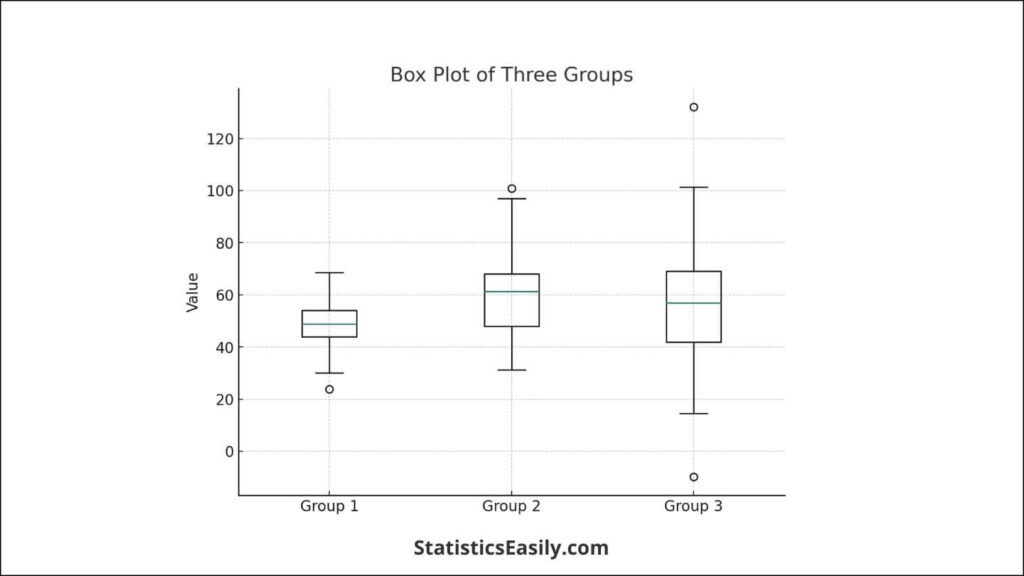
Visual Representation

Consider creating a box plot to visualize the distribution of your data across the groups. This can help in understanding the data and explaining the results.

---

How to Perform the Kruskal-Wallis Test in R

This guide provides a detailed, step-by-step tutorial on performing the Kruskal-Wallis Test using R, including calculating effect size and conducting post-hoc tests for multiple comparisons.

Preparation of Data:

1. Data Input: Begin by ensuring your data is formatted correctly in R. Typically, you will have one column representing the independent variable (grouping factor) and another for the dependent variable (scores or measurements you wish to compare).

# Sample data creation
set.seed(123)  # For reproducibility
group <- factor(rep(c("Group1", "Group2", "Group3"), each = 20))
score <- c(rnorm(20, mean = 50, sd = 10), 
           rnorm(20, mean = 55, sd = 15), 
           rnorm(20, mean = 60, sd = 20))
data <- data.frame(group, score)

2. Data Inspection: Visualizing and inspecting your data before running the test is crucial. Use boxplots to assess the distribution across groups.

# Data visualization
boxplot(score ~ group, data = data, main = "Group Comparison", ylab = "Scores", xlab = "Group")

Performing Kruskal-Wallis Test:

1. Run the Test: Utilize the kruskal.test() function in R, specifying your dependent and independent variables.

# Kruskal-Wallis Test
kruskal_test_result <- kruskal.test(score ~ group, data = data)
print(kruskal_test_result)

2. Interpret Results: The output will provide the Kruskal-Wallis statistic and the associated p-value. A significant p-value (typically < 0.05) indicates a difference in medians across the groups.

Effect Size Calculation:

1. Compute Eta-squared: While Kruskal-Wallis test does not directly provide an effect size, eta-squared (η²) can be used as an estimate.

# Effect size calculation
eta_squared <- kruskal_test_result$statistic / length(data$score)
print(eta_squared)

Post-Hoc Analysis:

1. Perform Post-Hoc Tests: If the Kruskal-Wallis test is significant, you may need to perform post-hoc tests to identify which groups differ. The pairwise.wilcox.test() function with a Bonferroni correction can be used for this purpose.

# Post-hoc analysis
post_hoc_result <- pairwise.wilcox.test(data$score, data$group, p.adjust.method = "bonferroni")
print(post_hoc_result)

2. Interpret Post-Hoc Results: This will provide pairwise comparisons between groups, highlighting significant differences.

---

Interpreting the Results of Kruskal-Wallis Test

Understanding the results of the Kruskal-Wallis Test involves dissecting several crucial components, including the H statistic, p-values, and effect sizes. Additionally, when significant differences are identified, post-hoc analyses are essential for pinpointing specific group differences. This section aims to clarify these elements, providing a comprehensive overview of the analysis outcomes.

H Statistic and P-values

The H statistic is the core outcome of the Kruskal-Wallis Test, signifying the variance among the ranks across different groups. A larger H value suggests a more pronounced difference between group medians. To decipher this statistic:

• The H value is compared against a critical value from the Chi-square distribution, factoring in the degrees of freedom (number of groups minus one).
• The p-value associated with the H statistic indicates the probability of observing the given result, or more extreme, under the null hypothesis. A p-value below the predefined alpha level (usually 0.05) indicates a statistically significant difference among at least one pair of group medians.

Effect Sizes

Effect sizes quantify the magnitude of differences observed, offering a dimension of interpretation beyond statistical significance. For the Kruskal-Wallis Test, eta squared (η²) is a commonly utilized measure, reflecting the variance in ranks attributable to group differences. The interpretation of eta-squared values is as follows:

• Small effect: η² ≈ 0.01
• Medium effect: η² ≈ 0.06
• Large effect: η² ≈ 0.14

Multiple Comparisons and Post-Hoc Tests

Significant findings from the Kruskal-Wallis Test necessitate further examination through post-hoc tests to identify distinct group differences. These tests include Dunn’s, Nemenyi’s, and Conover’s, each tailored for specific conditions and data types. Critical points for conducting posthoc analyses are:

• Choose a post-hoc test that aligns with the study’s objectives and data attributes.
• These tests inherently adjust for the risk of Type I errors due to multiple comparisons, ensuring the integrity of the inferential process.

Common Pitfalls and Avoidance Strategies

• Overemphasis on Significance: A significant p-value doesn’t automatically imply a meaningful or large effect. It’s vital to integrate effect size considerations for a balanced interpretation.
• Distribution Assumptions: Although the Kruskal-Wallis Test is less assumption-bound than its parametric counterparts, it ideally requires comparable distribution shapes across groups, barring median differences. Ensuring this similarity enhances the test’s validity.

By precisely navigating these components, researchers can draw accurate and meaningful conclusions from the Kruskal-Wallis Test, enriching the understanding of their data’s underlying patterns and relationships.

---

Case Studies and Applications

The Kruskal-Wallis Test is a powerful non-parametric method for comparing three or more independent groups. This section presents real-world applications and hypothetical case studies to illustrate the efficacy and insights derived from utilizing the Kruskal-Wallis Test.

Real-World Application: Environmental Science

In an environmental study, researchers aimed to assess the impact of industrial pollution on the growth rates of specific plant species across multiple sites. The sites were categorized into three groups based on their proximity to industrial areas: high pollution, moderate pollution, and low pollution zones. Given the non-normal distribution of growth rates and the ordinal nature of the data, the Kruskal-Wallis Test was employed.

The test revealed a significant difference in median growth rates among the three groups (H statistic significant at p < 0.05), indicating that pollution levels significantly affect plant growth. This insight led to targeted environmental policies focusing on reducing industrial emissions in critical areas.

Hypothetical Example: Healthcare Research

Consider a hypothetical study in healthcare where researchers investigate the effectiveness of three different treatment protocols for chronic disease. Patients are randomly assigned to one of the three treatment groups, and the outcome measure is the improvement in quality of life, scored on an ordinal scale.

Utilizing the Kruskal-Wallis Test, researchers find a statistically significant difference in the median improvement scores across the treatment groups. Further post-hoc analysis identifies which specific treatments differ significantly, guiding medical professionals toward more effective treatment protocols.

---

Conclusion

Throughout this article, we have explored the Kruskal-Wallis Test, emphasizing its critical role in statistical analysis when dealing with non-parametric data across multiple groups. This test’s value lies in its ability to handle data that do not meet the assumptions of normality, providing a robust alternative to traditional ANOVA. Its versatility is demonstrated through various applications, from environmental science to healthcare, where it aids in deriving meaningful insights that guide decision-making and policy development. The Kruskal-Wallis Test stands as a testament to the pursuit of truth, enabling researchers to uncover the underlying patterns in data, thereby contributing to the greater good by informing evidence-based practices.

---

Recommended Articles

Discover more cutting-edge statistical techniques and their applications by exploring our collection of in-depth articles on our blog.

1. Mastering One-Way ANOVA: A Comprehensive Guide for Beginners
2. Mastering the Mann-Whitney U Test: A Comprehensive Guide
3. Common Mistakes to Avoid in One-Way ANOVA Analysis
4. Non-Parametric Statistics: A Comprehensive Guide
5. MANOVA: A Practical Guide for Data Scientists

---

Frequently Asked Questions (FAQs)

Q1: What is the Kruskal-Wallis Test? The Kruskal-Wallis Test is a non-parametric statistical method used to compare medians across three or more independent groups. It’s beneficial when data do not meet the assumptions required for parametric tests like the one-way ANOVA.

Q2: When should the Kruskal-Wallis Test be used? This test is suitable for non-normal distributions, ordinal data, heterogeneous variances, and small sample sizes where traditional parametric assumptions cannot be met.

Q3: How does the Kruskal-Wallis Test differ from ANOVA? Unlike ANOVA, the Kruskal-Wallis Test does not assume a normal data distribution or variance homogeneity. It ranks the data and compares the sums of these ranks between groups, making it ideal for non-normal distributions and ordinal data.

Q4: What are the assumptions of the Kruskal-Wallis Test? The main assumptions include the dependent variable being continuous or ordinal, the independent variable consisting of two or more categorical, independent groups, and the observations across groups being independent.

Q5: Can the Kruskal-Wallis Test be used for post-hoc analysis? Yes, upon finding significant results, post-hoc tests like Dunn’s Test, Nemenyi Test, Conover’s Test, Dwass-Steel-Critchlow-Fligner Test, and Mann-Whitney U Test (with adjustments) can be conducted to identify specific group differences.

Q6: How are effect sizes calculated in the Kruskal-Wallis Test? Effect sizes can be quantified using adapted Eta Squared (η²), Epsilon Squared (ε²), an adapted version of Cohen’s d for non-parametric use, and Rank-Biserial Correlation, providing insights into the magnitude of group differences.

Q7: What are some practical applications of the Kruskal-Wallis Test? This test is widely used in clinical research, environmental science, marketing studies, and educational research, mainly when dealing with ordinal data, non-normal distributions, or small sample sizes.

Q8: How is the data analyzed in the Kruskal-Wallis Test? Data is ranked across all groups, and the test evaluates whether the distribution of ranks differs significantly across the groups, focusing on median differences rather than mean differences.

Q9: What should be considered when interpreting the results of the Kruskal-Wallis Test? While the test indicates whether group differences are statistically significant, it does not specify where they lie. Post-hoc tests are necessary for detailed pairwise comparisons.

Q10: Are there limitations to the Kruskal-Wallis Test? Yes, the test does not provide information on mean differences and requires subsequent post-hoc analyses for detailed insights. It also does not accommodate paired data or repeated measures.