
Assumptions in Linear Regression: A Comprehensive Guide
You will learn the fundamentals of the assumptions in linear regression and how to validate them using real-world examples for practical data analysis.
Highlights
- Linear regression is a widely used predictive modeling technique for understanding relationships between variables.
- The normality of residuals helps ensure unbiased predictions and trustworthy confidence intervals in linear regression.
- Homoscedasticity guarantees that the model’s predictions have consistent precision across different values.
- Identifying and addressing multicollinearity improves the stability and interpretability of your regression model.
- Data preprocessing and transformation techniques, such as scaling and normalization, can mitigate potential issues in linear regression.
Linear regression is a technique to model and predict the relationship between a target variable and one or more input variables.
It helps us understand how a change in the input variables affects the target variable.
Linear regression assumes that a straight line can represent this relationship.
For example, let’s say you want to estimate the cost of a property considering its size (measured in square footage) and age (in years).
In this case, the price of the house is the target variable, and the size and age are the input variables.
Using linear regression, you can estimate the effect of size and age on the price of the house.
Assumptions in Linear Regression
Six main assumptions in linear regression need to be satisfied for the model to be reliable and valid. These assumptions are:
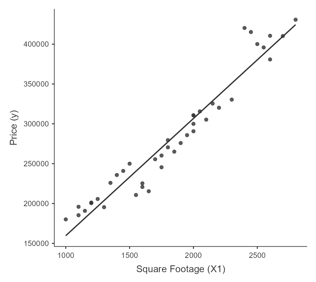
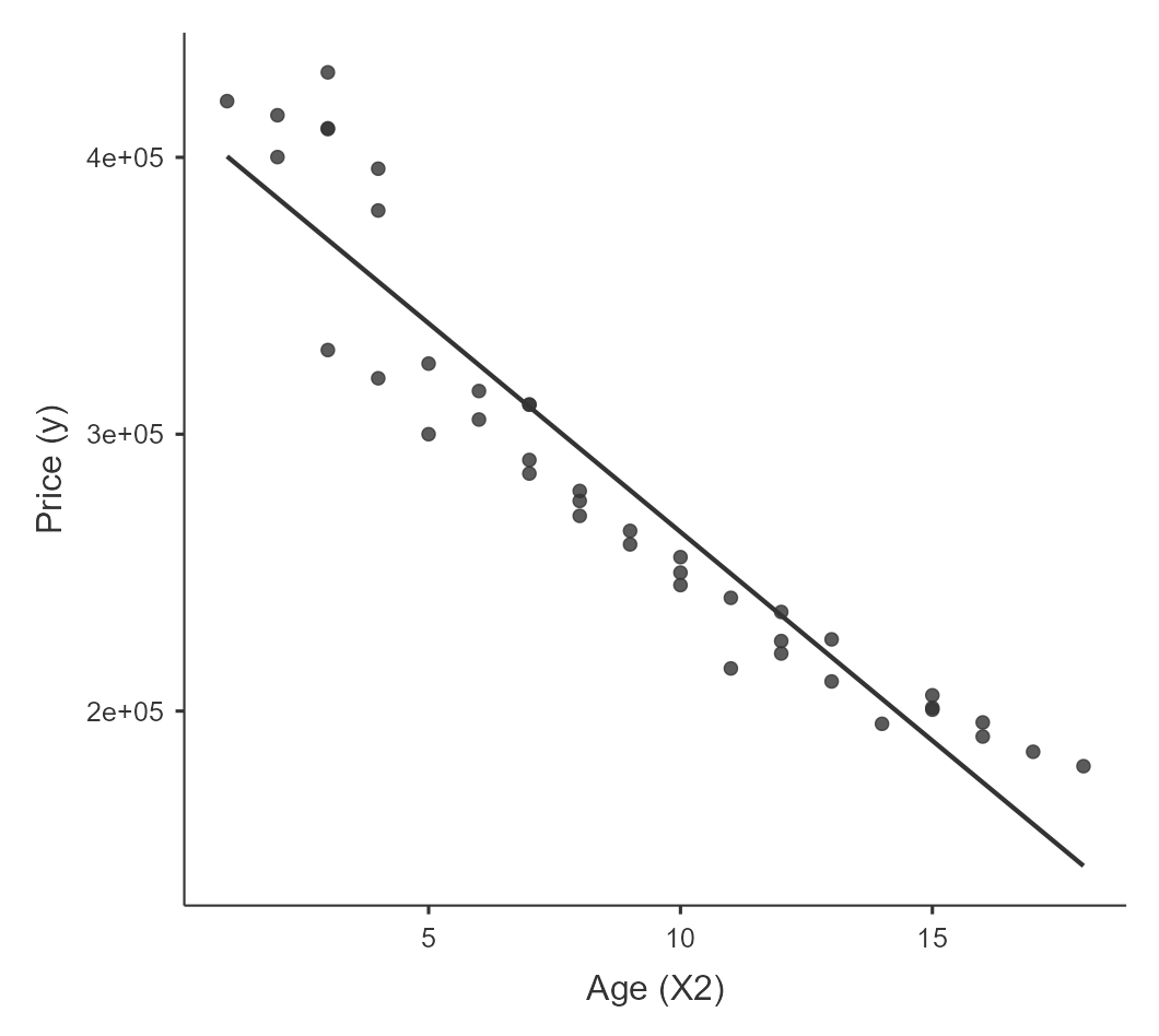
1. Linearity
This assumption states a linear relationship exists between the dependent and independent variables. In other words, the change in the dependent variable should be proportional to the change in the independent variables. Linearity can be assessed using scatterplots or by examining the residuals.
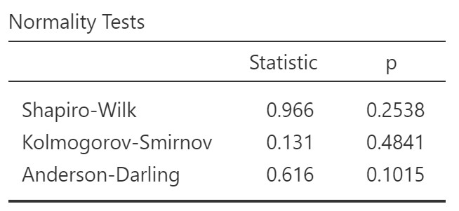
2. Normality of errors
The residuals should follow a normal distribution with a mean of zero. This assumption is essential for proper hypothesis testing and constructing confidence intervals. The normality of errors can be assessed using visual methods, such as a histogram or a Q-Q plot, or through statistical tests, like the Shapiro-Wilk test or the Kolmogorov-Smirnov test.
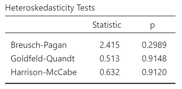
3. Homoscedasticity
This assumption states that the residuals’ variance should be constant across all independent variable levels. In other words, the residuals’ spread should be similar for all values of the independent variables. Heteroscedasticity, violating this assumption, can be identified using scatterplots of the residuals or formal tests like the Breusch-Pagan test.
4. Independence of errors
This assumption states that the dataset observations should be independent of each other. Observations may depend on each other when working with time series or spatial data due to their temporal or spatial proximity. Violating this assumption can lead to biased estimates and unreliable predictions. Specialized models like time series or spatial models may be more appropriate in such cases.
5. Absence of multicollinearity (Multiple Linear Regression)
Multicollinearity takes place when two or more independent variables in the linear regression model are highly correlated, making it challenging to establish the precise effect of each variable on the dependent variable. Multicollinearity can lead to unstable estimates, inflated standard errors, and difficulty interpreting coefficients. You can use the variance inflation factor (VIF) or correlation matrix to detect multicollinearity. If multicollinearity is present, consider dropping one of the correlated variables, combining the correlated variables, or using techniques like principal component analysis (PCA) or ridge regression.
6. Independence of observations
This assumption states that the dataset observations should be independent of each other. Observations may depend on each other when working with time series or spatial data due to their temporal or spatial proximity. Violating this assumption can lead to biased estimates and unreliable predictions. Specialized models like time series or spatial models may be more appropriate in such cases.
By ensuring that these assumptions are met, you can increase your linear regression models’ accuracy, reliability, and interpretability. If any assumptions are violated, it may be necessary to apply data transformations, use alternative modeling techniques, or consider other approaches to address the issues.

❓ Confused by Data Analysis? Our Comprehensive Guide Will Make It Crystal Clear
| Assumptions | Description |
|---|---|
| Linearity | Linear relationship between dependent and independent variables, checked using scatterplots |
| Normality | Normal distribution of residuals, assessed using Shapiro-Wilk test |
| Homoscedasticity | Constant variance in error terms, evaluated using Breusch-Pagan test |
| Independence of errors | Independent error terms, verified using Durbin-Watson test |
| Independence of observations | Independently collected data points without autocorrelation |
| Absence of multicollinearity | No multicollinearity among independent variables, determined using VIF and Tolerance measures |
Practical Example
Here is a demonstration of a linear regression model problem with two independent variables and one dependent variable.
In this example, we will model the relationship between a house’s square footage and age with its selling price.
The dataset contains the square footage, age, and selling price of 40 houses.
We will use multiple linear regression to estimate the effects of square footage and age on selling price.
Here is a table with the data that you can copy and paste:
| House | SquareFootage | Age | Price |
|---|---|---|---|
| 1 | 1500 | 10 | 250000.50 |
| 2 | 2000 | 5 | 300000.75 |
| 3 | 1200 | 15 | 200500.25 |
| 4 | 2500 | 2 | 400100.80 |
| 5 | 1800 | 8 | 270500.55 |
| 6 | 1600 | 12 | 220800.60 |
| 7 | 2200 | 4 | 320200.10 |
| 8 | 2400 | 1 | 420300.90 |
| 9 | 1000 | 18 | 180100.15 |
| 10 | 2000 | 7 | 290700.40 |
| 11 | 1450 | 11 | 240900.65 |
| 12 | 2050 | 6 | 315600.20 |
| 13 | 1150 | 16 | 190800.75 |
| 14 | 2600 | 3 | 410500.50 |
| 15 | 1750 | 9 | 260200.55 |
| 16 | 1550 | 13 | 210700.85 |
| 17 | 2300 | 3 | 330400.45 |
| 18 | 2450 | 2 | 415200.90 |
| 19 | 1100 | 17 | 185300.65 |
| 20 | 1900 | 8 | 275900.80 |
| 21 | 1400 | 12 | 235800.55 |
| 22 | 2100 | 6 | 305300.40 |
| 23 | 1300 | 14 | 195400.25 |
| 24 | 2700 | 3 | 410200.75 |
| 25 | 1700 | 10 | 255600.20 |
| 26 | 1650 | 11 | 215400.60 |
| 27 | 2150 | 5 | 325500.50 |
| 28 | 1250 | 15 | 205700.85 |
| 29 | 2550 | 4 | 395900.90 |
| 30 | 1850 | 9 | 265100.65 |
| 31 | 1350 | 13 | 225900.40 |
| 32 | 1950 | 7 | 285800.15 |
| 33 | 1100 | 16 | 195900.80 |
| 34 | 2800 | 3 | 430700.55 |
| 35 | 1750 | 10 | 245500.20 |
| 36 | 1600 | 12 | 225300.10 |
| 37 | 2000 | 7 | 310700.50 |
| 37 | 2000 | 7 | 310700.50 |
| 38 | 1200 | 15 | 201200.90 |
| 39 | 2600 | 4 | 380800.65 |
| 40 | 1800 | 8 | 279500.25 |
1. Linearity
Assess the linearity assumption by visually inspecting the scatterplot of the dependent variable against each independent variable for a discernible linear pattern.
2. Normality of errors
Evaluate the normality assumption by conducting the Shapiro-Wilk test, which assesses the residuals’ distribution for significant deviations from a normal distribution.
In the Shapiro-Wilk test, a high p-value (typically above 0.05) indicates that the residuals’ distribution does not significantly differ from a normal distribution.
3. Homoscedasticity
Assess the homoscedasticity assumption by performing the Breusch-Pagan test, which checks for non-constant variance in the error terms.
A high p-value (typically above 0.05) suggests that the data exhibits homoscedasticity, with constant variance across different values.
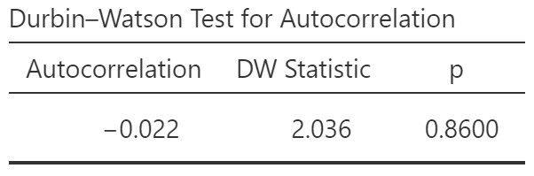
4. Independence of errors
A Durbin-Watson statistic close to 2 suggests that the errors are independent, with minimal autocorrelation present.
Values below or above 2 indicate positive or negative autocorrelation, respectively.
The p-value signifies that the DW statistic is not significantly different from 2.
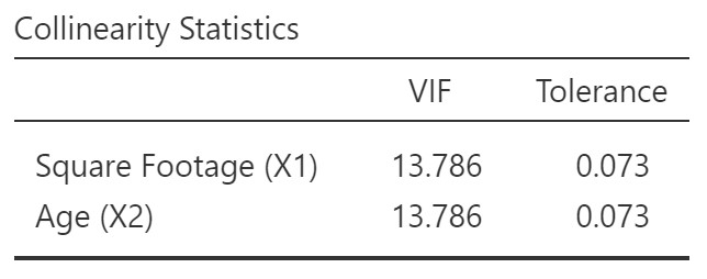
5. Absence of multicollinearity
Assess the absence of multicollinearity using Variance Inflation Factor (VIF) and Tolerance measures. Low VIF values (typically below 10) and high Tolerance values (above 0.1) indicate that multicollinearity is not a significant concern in the regression model.
Our data indicate the presence of multicollinearity between the variables age and square footage. We will need to remove one of them. The variable to be removed can be determined in various ways, such as testing with simple linear regressions to see which fits the model better or deciding based on the underlying theory.
6. Independence of observations
To avoid violating the independence of observations assumption, ensure that your data points are collected independently and do not exhibit autocorrelation, which can be assessed using the Durbin-Watson test.
Conclusion
It is crucial to examine and address these assumptions when building a linear regression model to ensure validity, reliability, and interpretability.
By understanding and verifying the six assumptions — linearity, independence of errors, homoscedasticity, normality of errors, independence of observations, and absence of multicollinearity — you can build more accurate and reliable models, leading to better decision-making and improved understanding of the relationships between variables in your data.
Seize the opportunity to access FREE samples from our newly released digital book and unleash your potential.
Dive deep into mastering advanced data analysis methods, determining the perfect sample size, and communicating results effectively, clearly, and concisely.
Click the link to uncover a wealth of knowledge: Applied Statistics: Data Analysis.