
How to Calculate Residuals in Regression Analysis?
You will learn the precise methods to calculate and interpret residuals in regression analysis for enhanced data insights.
Introduction
Understanding linear regression and the role of residuals is crucial in regression analysis. In this article, we delve into the fundamentals of linear regression, a popular statistical method used for modeling the relationship between a dependent variable and one or more independent variables. By exploring this concept, we set the groundwork for a deeper comprehension of regression analysis.
The importance of calculating residuals in regression analysis cannot be overstated. Residuals, the differences between the observed values and the values predicted by the regression model, are key indicators of the model’s accuracy and effectiveness. They provide valuable insights into the model’s performance, highlighting whether the model adequately captures the underlying relationship in the data.
Highlights
- Residuals reveal the difference between observed and predicted values in regression models.
- Effective residual analysis improves the accuracy of regression models.
- Visualizing residuals helps identify patterns and model deficiencies.
- The correct interpretation of residuals is crucial for diagnosing model fit.
- Advanced techniques address non-linearity and heteroscedasticity in residuals.
Ad Title
Ad description. Lorem ipsum dolor sit amet, consectetur adipiscing elit.
The Concept of Residuals
In regression analysis, understanding the concept of residuals is fundamental. A residual is the difference between an observed value and the value predicted by a regression model. This discrepancy is not just a simple error; it holds significant importance in evaluating the effectiveness of a model.
Residuals serve as critical indicators of model accuracy. They provide insights into how well the model captures the underlying data trends. The residuals will generally be small and randomly distributed if a model is accurate. Large or patterned residuals, on the other hand, indicate that the model may not be adequately representing the data.
Step-by-Step Guide to Calculating Residuals
Calculating residuals in regression analysis is a straightforward yet vital process. First, let’s define the formula for a residual: the difference between the observed value (y) and the predicted value (ŷ) for each data point. Mathematically, it’s expressed as e=y−y^.
To illustrate this process, consider a simple linear regression model and a dataset with 10 data points. Calculate the predicted value using the regression equation for each point, then compute the residual by subtracting this predicted value from the observed value.
A detailed example will follow, using a hypothetical dataset to perform these calculations. This example will include creating a table listing the observed values, the predicted values, and the calculated residuals for each data point. We’ll plot these residuals to visually assess their distribution and any patterns that may suggest model inadequacies. This practical demonstration aims to provide a clear understanding of how to calculate and interpret residuals effectively.
Through this step-by-step guide, readers will gain hands-on knowledge of residual analysis, a key component in refining regression models and enhancing their predictive accuracy.
Example
We’ve created a hypothetical dataset with 10 data points for our detailed example. Using this dataset, we conducted a simple linear regression analysis, calculated the predicted values, and derived the residuals. The process unfolded as follows:
1. Data Creation: The dataset consists of an independent variable (X) and a dependent variable (y). The independent variable values range randomly from 0 to 10, and the dependent variable values are generated to have a linear relationship with some added random noise for realism.
| Independent Variable (X) | Dependent Variable (y) |
|---|---|
| 5.488135 | 14.008425 |
| 7.151894 | 20.788281 |
| 6.027634 | 16.591160 |
| 5.448832 | 13.865430 |
| 4.236548 | 11.479096 |
| 6.458941 | 16.814701 |
| 4.375872 | 13.927838 |
| 8.917730 | 21.884008 |
| 9.636628 | 24.717704 |
| 3.834415 | 7.877846 |
2. Linear Regression Model: A linear regression model was fitted to this data. The model’s equation can be represented as y=β0+β1X+ϵ, where β0 (intercept) is approximately 0.71, and β1 (coefficient) is about 2.52.
y = 0.71 + 2.52X + ϵ
3. Predicted Values and Residuals: We calculated the predicted value using the regression model and then determined each data point’s residual (the difference between the observed and the predicted value).
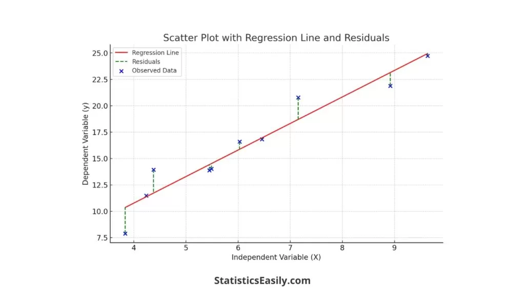
Here is a summary table showing the observed values, predicted values, and the calculated residuals for each data point:
| Observed Values | Predicted Values | Residuals |
|---|---|---|
| 14.01 | 14.51 | -0.50 |
| 20.79 | 18.70 | 2.09 |
| 16.59 | 15.87 | 0.72 |
| 13.87 | 14.41 | -0.55 |
| 11.48 | 11.36 | 0.12 |
| 16.81 | 16.95 | -0.14 |
| 13.93 | 11.71 | 2.21 |
| 21.88 | 23.14 | -1.25 |
| 24.72 | 24.95 | -0.23 |
| 7.88 | 10.35 | -2.47 |
Residual Plot: The residual plot visually represents the residuals against the independent variable. A horizontal line at zero indicates where the residuals would be if the model perfectly predicted the values. The scatter of points around this line helps assess the model’s performance. We can observe how the residuals are distributed in the plot and look for patterns that might indicate model deficiencies.
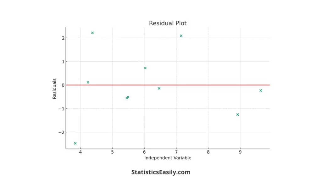
This step-by-step guide, with its practical example and visual aids, illustrates the importance of calculating and analyzing residuals in regression models. It enhances the understanding of the concept and demonstrates the application in a real-world context.
Interpreting Residuals
Residuals, the deviations of the observed values from the predicted values, can indicate how well a model fits the data. They are the unexplained portion of the model, offering a window into its limitations and potential improvements.
When analyzing residuals, one looks for randomness. Ideally, residuals should appear randomly scattered around the horizontal axis, indicating that the model’s predictions are unbiased and the variance is consistent across all independent variable levels. Systematic patterns in the residuals, such as a curve or clustering, may suggest problems with the model, such as non-linearity or heteroscedasticity.
Diagnosing issues in regression models using residuals involves several steps:
1. Visual Inspection: Creating a residual plot is the first step. This graph can help spot obvious issues like patterns or outliers. If the residuals do not appear to be randomly distributed, this is a sign that the model may not be capturing all the relevant information.
2. Statistical Tests: Beyond visual inspection, statistical tests can provide evidence of autocorrelation (where residuals in one period are related to residuals in another) or heteroscedasticity (where residuals have non-constant variance).
3. Model Comparison: Sometimes, comparing residuals between different models can help diagnose issues. If one model’s residuals show less pattern and are closer to zero, that model may better fit the data.
Visualizing Residuals
Visualizing residuals allows for the graphical representation of the errors between the observed and predicted values, providing an intuitive understanding of a regression model’s performance. By creating and interpreting residual plots, we can quickly identify any systematic deviations that suggest potential problems with the model.
Creating residual plots is typically one of the first steps in the residual analysis process. These plots are simple to generate using various statistical software tools and programming languages. Such a plot should ideally show residuals scattered randomly around the horizontal axis, suggesting that the regression model fits well.
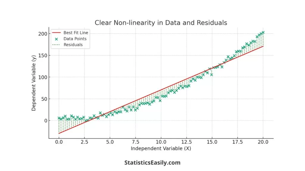
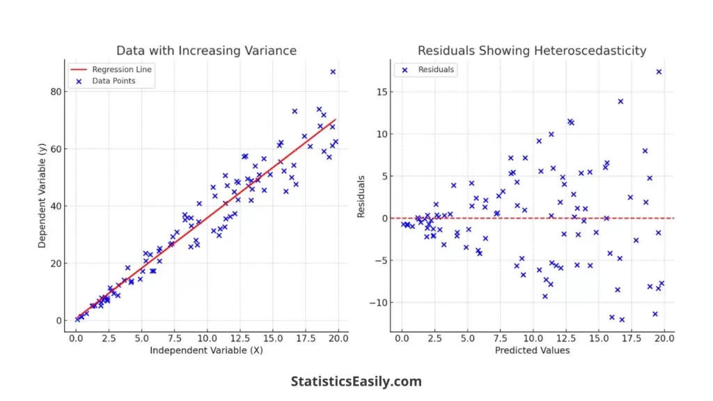
When interpreting residual plots, we look for the absence of patterns. Suppose residuals show a pattern, especially a discernible shape or trend. In that case, this is a sign that the regression model is not capturing some aspect of the relationship between variables. For example, a U-shaped pattern might suggest a non-linear model is more appropriate. Similarly, if the residuals increase or decrease with the predicted values, it might indicate heteroscedasticity.
Advanced Considerations
Two common issues that analysts encounter are non-linearity and heteroscedasticity in the data. Understanding and addressing these issues is essential for improving the accuracy and predictive power of the model.
Non-linearity occurs when a straight line cannot accurately describe the relationship between the independent and dependent variables. This can often be detected by a systematic pattern in the residuals, such as a curved or more complex shape. To address non-linearity, the transformation of the variables may be necessary. For instance, logging or squaring variables can help linearize the relationship, allowing for a better linear regression model fit.
On the other hand, heteroscedasticity is present when the residuals do not have constant variance across the range of predicted values. This issue can often be identified by a fan or cone-shaped pattern in the residual plot, where the spread of residuals increases with the magnitude of the predicted value. Heteroscedasticity can be problematic because it violates the assumption of the residuals’ homoscedasticity (constant variance), which underpins many of the statistical tests used in regression analysis. To deal with heteroscedasticity, one might consider using robust regression techniques or transforming the dependent variable to stabilize the variance.
Here are some tips for improving model fit using residual analysis:
1. Examine Residual Plots: Carefully analyze the residual plots for any patterns. If patterns are detected, consider using polynomial regression or other non-linear models.
2. Variable Transformation: Apply logarithmic, square root, or reciprocal transformations to the dependent or independent variables to correct non-linearity or heteroscedasticity.
3. Addition of Variables: Sometimes, including another variable or an interaction term can help account for the effects causing non-linearity or heteroscedasticity.
4. Alternative Models: If the residuals indicate that a linear model is inappropriate, explore non-linear models that may provide a better fit.
5. Weighted Least Squares: For heteroscedastic data, weighted least squares regression can help by assigning weights to data points based on the variance of their residuals.
Conclusion
Residuals, the discrepancies between observed and predicted values, are not mere byproducts of predictive modeling but are integral in assessing the accuracy and appropriateness of a regression model. They shed light on the model’s capacity to encapsulate the underlying data trends, thereby ensuring the validity of the insights drawn from the analysis.
Throughout this article, we have underscored the vitality of calculating residuals, which reveals the nuanced difference between the observed and predicted values in regression models. We’ve seen that practical residual analysis improves the accuracy of regression models and aids in identifying patterns and deficiencies that might not be apparent on the surface.
The precise interpretation of residuals is indispensable for diagnosing model fit. This article has illustrated that advanced techniques, such as variable transformation and the adoption of robust regression methods, are necessary tools in the data scientist’s arsenal to address non-linearity and heteroscedasticity — common challenges in real-world data.
Ad Title
Ad description. Lorem ipsum dolor sit amet, consectetur adipiscing elit.
Recommended Articles
Discover more insights and advanced techniques in regression analysis by exploring our comprehensive collection of related articles on our blog.
- What’s Regression Analysis? A Comprehensive Guide for Beginners
- How to Report Simple Linear Regression Results in APA Style
- Assumptions in Linear Regression: A Comprehensive Guide
Frequently Asked Questions (FAQs)
Q1: What are residuals in regression analysis? Residuals are the differences between observed and predicted values in a regression model, crucial for assessing model accuracy.
Q2: Why are residuals crucial in regression models? They help identify how well the model fits the data and highlight areas for improvement.
Q3: How do you calculate residuals in regression? Subtract the predicted value from the actual observed value for each data point in your dataset.
Q4: What can patterns in residuals indicate? Patterns in residuals can reveal issues such as non-linearity, heteroscedasticity, or other model inaccuracies.
Q5: How do residuals enhance model accuracy? Analyzing residuals can lead to model refinement, ensuring more accurate predictions and insights.
Q6: What is the purpose of a residual plot? A residual plot visually assesses the distribution of residuals against predicted values, helping to identify any systematic errors.
Q7: Can residuals indicate overfitting? Yes, unusually large residuals may suggest overfitting, where the model captures noise instead of underlying patterns.
Q8: How are outliers identified using residuals? Significant large residuals often reveal outliers, differing markedly from other data points.
Q9: What does heteroscedasticity in residuals mean? Heteroscedasticity occurs when residuals show non-constant variability, indicating potential issues in model assumptions.
Q10: How can you address non-linearity in residuals? Addressing non-linearity might involve transforming variables or adopting more complex, non-linear models.