RM ANOVA: The Definitive Guide to Understanding Within-Subject Variability

You will learn the transformative approach RM ANOVA brings to within-subject variability analysis in research.

---

Introduction

Repeated Measures ANOVA (RM ANOVA) is a cornerstone in statistical analysis, particularly in studies where the same subjects undergo multiple measurements under varying conditions. This technique illuminates the nuances of within-subject variability, offering a lens through which to view how individual responses change over time or in different contexts. The essence of this article is to demystify RM ANOVA, guiding you through its conceptual underpinnings to practical applications. By the end, you’ll gain a thorough understanding of this powerful analytical tool and the ability to apply it to your research, enhancing the rigor and depth of your analyses. This guide aims to equip you with the knowledge to leverage RM ANOVA effectively, ensuring your research stands on a foundation of precision and clarity.

---

Highlights

1. RM ANOVA delineates within-subject effects with unmatched precision.
2. Statistical assumptions of RM ANOVA ensure rigorous data analysis.
3. Step-by-step RM ANOVA guide enhances analytical proficiency.
4. Interpreting RM ANOVA results unlocks deeper data insights.
5. Case studies illustrate RM ANOVA’s versatility across fields.

---

Understanding RM ANOVA

Repeated Measures ANOVA is a specialized form of ANOVA explicitly designed for situations where multiple measurements are taken on the same subjects under different conditions or over time. This contrasts with traditional ANOVA, which compares means across different groups, assuming independence between observations. RM ANOVA accounts for the correlation between these repeated measurements, providing a more accurate analysis by considering the within-subject variability.

The application of RM ANOVA is particularly relevant in longitudinal studies, clinical trials, or any research scenario where the same subjects are observed under various conditions or times. This relevance stems from its ability to control for individual differences that might otherwise confound the results, thereby offering a clearer picture of the effect of the independent variable on the dependent variable. By utilizing RM ANOVA, researchers can effectively isolate and understand the changes within subjects across different conditions, making it an invaluable tool in statistical analysis, where the intricacy of data demands robust and nuanced analytical approaches.

Within the framework of Repeated Measures ANOVA, several types cater to different research designs and data structures. These include:

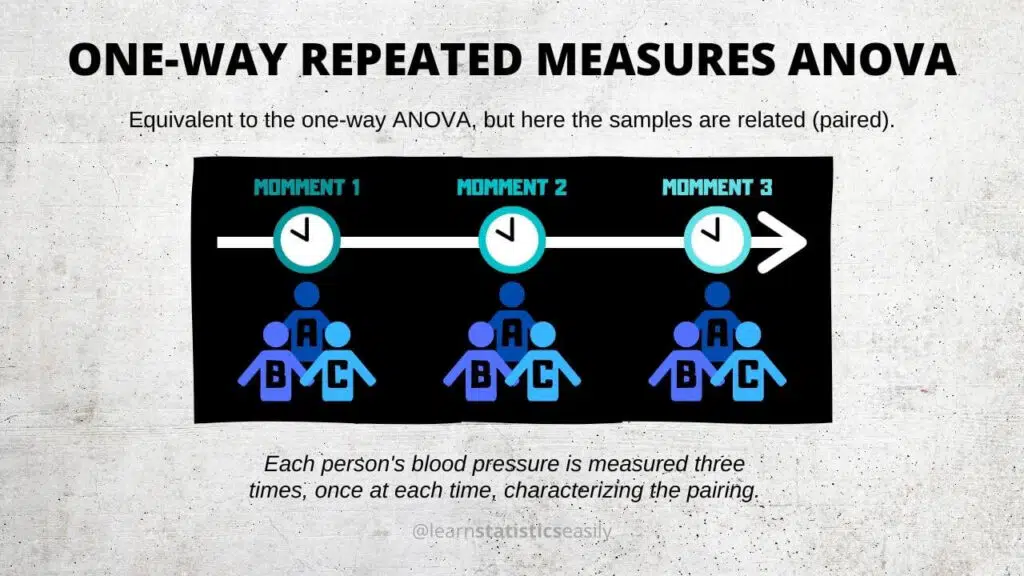
One-Way RM ANOVA: Used when one within-subject factor (e.g., time) has multiple levels. This type assesses the effect of this single factor on the dependent variable across different time points or conditions.

Two-Way RM ANOVA: Applied when there are two within-subject factors, allowing researchers to examine the main effects of each factor and the interaction between them. This is particularly useful in studies where the effect of one factor may depend on the level of the other factor.

Mixed ANOVA (Split-Plot ANOVA): Incorporates within-subjects (repeated measures) and between-subjects factors. This type is ideal for experiments where some factors vary within subjects over time or conditions, while other factors vary between different groups of subjects.

Each of these RM ANOVA types offers unique insights into data, enabling researchers to tailor their statistical approach to the specific needs of their study, thereby enhancing the depth and accuracy of their analyses.

---

RM ANOVA Theoretical Foundations

The statistical theory underpinning Repeated Measures ANOVA is founded on analyzing variances within subjects to understand the effects of different conditions or time points on a dependent variable. This contrasts with traditional ANOVA, which focuses on between-group variances, neglecting the correlation inherent in repeated measures on the same subjects.

Key Assumptions:

Sphericity: RM ANOVA presupposes that the variances of the differences between all combinations of related groups are equal. This assumption, unique to repeated measures designs, ensures the validity of the F-ratio used in hypothesis testing.

Normality: The distribution of residuals (differences between observed and predicted values by the model) should approximate a normal distribution for accurate p-values.

Independence: While measurements within subjects are expected to be correlated, the assumption of independence pertains to the lack of correlation between the different subjects themselves.

Hypothesis Testing in RM ANOVA:

RM ANOVA tests the null hypothesis that the mean differences between related groups are zero. When the F-ratio, derived from the ratio of mean squares due to the treatment to the mean squares due to error, is significantly large, the null hypothesis is rejected, indicating significant differences between the means of the groups.

Illustrative Example:

Consider a study investigating the effect of a new diet regimen on weight loss over three months, with measurements taken monthly. In this case, RM ANOVA would compare the weight measurements across the three-time points within the same group of subjects to determine if significant weight changes occurred due to the diet.

---

Step-by-Step Guide to Performing RM ANOVA

Performing a Repeated Measures ANOVA in R involves a comprehensive approach that starts from data collection to the analysis phase. This guide will take you through generating example data and descriptive statistics, creating an appropriate graph, and conducting the RM ANOVA with detailed analysis, including test statistics, post-hoc analysis, p-values, effect sizes, and other relevant metrics.

1. Data Generation for Example

First, we must simulate a dataset representing repeated measurements for subjects across different time points or conditions. Here’s how you can generate example data:

set.seed(42)  # Ensures reproducibility
subjects <- 10
times <- c("Time1", "Time2", "Time3")  # Time points
data <- data.frame(matrix(rnorm(subjects * length(times), mean=5, sd=1.5), ncol=length(times)))
colnames(data) <- times
data$Subject <- paste("Subject", 1:subjects, sep="")

Note: This code block creates a 10×3 matrix where rows represent subjects and columns represent different time points.

2. Descriptive Statistics

Before diving into RM ANOVA, it’s crucial to understand your data. You can use the following R code to obtain descriptive statistics:

summary(data[, -ncol(data)])  # Summary for each time point
sapply(data[, -ncol(data)], sd)  # Standard deviation for each time point

3. Data Visualization

A graph can provide insights into your data’s distribution across time points. Here’s how to create a boxplot in R:

data_long <- reshape2::melt(data, id.vars = "Subject")
boxplot(value ~ variable, data = data_long, main = "Scores Over Time", xlab = "Time", ylab = "Scores", col = "lightblue")

4. Conducting RM ANOVA

Now, let’s move on to the primary analysis part using the ‘aov’ function in R, which includes calculating the test statistics, p-values, and effect sizes.

data_long$Subject <- factor(data_long$Subject)  # Ensure 'Subject' is a factor
rm_anova <- aov(value ~ variable + Error(Subject/variable), data = data_long)
summary(rm_anova)

Note: This code reshapes the data into a long format suitable for ‘aov’ and conducts the RM ANOVA.

5. Post-Hoc Analysis

If your RM ANOVA results indicate significant effects, you might need to perform a posthoc analysis to understand pairwise differences:

# Install the 'multcomp' package if not already installed: install.packages("multcomp")
post_hoc <- multcomp::glht(rm_anova, linfct = multcomp::mcp(variable = "Tukey"))
summary(post_hoc)

6. Effect Size

Effect size, such as Partial Eta Squared, can be crucial for understanding the magnitude of observed effects. However, calculating this directly in R requires additional steps or packages, and it might look something like this:

# Install the 'sjstats' package if not already installed: install.packages("sjstats")
eta_squared <- sjstats::eta_sq(rm_anova)
print(eta_squared)

---

Interpreting RM ANOVA Results

Interpreting the results of a Repeated Measures ANOVA involves understanding the main effects, interactions between factors, and the outcomes of any post-hoc analyses conducted. This section will guide you through interpreting the RM ANOVA test output, supplemented by visual aids for enhanced comprehension.

Understanding Main Effects and Interactions

• Main Effects: These refer to the independent impact of each within-subject factor (e.g., Time) on the dependent variable (e.g., Scores). A significant main effect suggests that there are overall differences across the levels of this factor.
• Interactions in RM ANOVA: In the context of RM ANOVA, interactions typically involve a within-subject factor interacting with another within-subject factor (in a two-way RM ANOVA) or a between-subjects factor (in mixed models). Significant interactions indicate that the effect of one factor on the dependent variable changes across the levels of another factor.

Analyzing RM ANOVA Output

When you run RM ANOVA in R, the ‘summary()’ function provides the F-statistic, degrees of freedom, and p-value for each effect:

• F-statistic: Indicates the ratio of variance explained by the factor to the variance within groups. Higher values often indicate a more significant effect.
• Degrees of Freedom: Reflects the number of levels in the factors and the number of subjects.
• P-value: Determines the significance of the effects. A p-value below the alpha level (commonly set at 0.05) suggests that the effect is statistically significant.

Effect Size

• Effect Size (Partial Eta Squared): Provides a measure of how much variance in the dependent variable is explained by a factor accounting for the total variance. It’s calculated as the sum of squares for the effect divided by the total sum of squares. Higher values indicate a larger effect.

Post-Hoc Analysis

If significant effects are found, post-hoc analyses help pinpoint where the differences lie:

• Use methods like Tukey’s HSD for pairwise comparisons between levels of a significant factor.
• Each pairwise comparison will have its p-value, indicating whether those specific levels differ significantly.

Visual Aids

• Line Graphs: Plotting the mean scores for each level of a within-subject factor against each other can visually depict changes over time or conditions. Lines between points help illustrate interactions between factors.
• Boxplots: Provide a distributional view of the scores at each level, offering insights into variability and outliers within the data.

---

Case Studies and Applications

Repeated Measures ANOVA has been a pivotal tool in various research fields, allowing scientists to unravel the complexities of within-subject variability across multiple conditions or time points. This section highlights real-world applications of RM ANOVA, demonstrating its versatility and critical role in advancing our understanding of psychology, medicine, and biology.

Psychology: Understanding Cognitive Changes

In a landmark study on cognitive behavioral therapy (CBT) for anxiety, researchers utilized RM ANOVA to assess changes in anxiety levels across several treatment sessions. Subjects were evaluated at multiple points during the treatment, allowing the researchers to discern the therapy’s effectiveness over time. RM ANOVA revealed significant reductions in anxiety scores from the initial session to the conclusion, showcasing the therapy’s efficacy.

Medicine: Evaluating Treatment Efficacy

A clinical trial investigating a new drug’s impact on blood pressure provided insightful data through RM ANOVA. Patients’ blood pressure readings were taken at baseline, mid-treatment, and post-treatment phases. RM ANOVA was employed to analyze these repeated measurements, identifying a statistically significant decrease in blood pressure, which underscored the drug’s potential benefits.

Biology: Monitoring Environmental Effects on Plant Growth

In an ecological study, biologists applied RM ANOVA to examine the effects of varying light conditions on plant growth rates. By measuring growth at consistent intervals under different light exposures, they could ascertain the optimal conditions for plant development. The RM ANOVA results highlighted specific light conditions that significantly enhanced growth, providing valuable insights for agricultural practices.

Neuroscience: Tracking Brain Activity Changes

Neuroscientists often turn to RM ANOVA to analyze brain activity changes in response to stimuli. Participants’ brain scans were assessed while exposed to various emotional triggers in a study focused on neural responses to emotional stimuli. RM ANOVA enabled the researchers to pinpoint regions in the brain that showed significant activity changes, contributing to our understanding of emotional processing.

Sports Science: Assessing Training Program Outcomes

In sports science, RM ANOVA helps evaluate the effectiveness of training programs. An investigation into a new high-intensity interval training (HIIT) regimen measured athletes’ performance metrics at several intervals throughout the program. The analysis provided by RM ANOVA revealed significant improvements in endurance and strength, validating the training regimen’s efficacy.

---

Common Pitfalls and How to Avoid Them

When applying Repeated Measures ANOVA, researchers often encounter several common pitfalls that can compromise the integrity and validity of their findings. One can conduct more robust and reliable data analyses by recognizing these potential issues and adhering to best practices.

Violation of Assumptions

One of the most significant challenges in RM ANOVA is ensuring that the data meet the necessary assumptions, including sphericity, normality, and independence of observations.

Sphericity: This assumption requires that the variances of the differences between all combinations of related groups are equal. Violating this assumption can lead to inflated Type I errors. To address this, use Mauchly’s test to check for sphericity, and if violated, apply corrections such as Greenhouse-Geisser or Huynh-Feldt adjustments.

Normality: RM ANOVA assumes that the residuals are normally distributed. Non-normal data can be transformed, or non-parametric alternatives can be considered for severely skewed distributions.

Independence: While repeated measures on the same subjects are inherently related, each subject’s measurements should be independent of others. Ensure the study design prevents contamination or crossover effects between subjects.

Inadequate Sample Size

Considering the within-subject design, RM ANOVA requires a sufficiently large sample to detect meaningful effects. Small sample sizes can lead to reduced statistical power, making it challenging to identify significant effects. Planning the study with a power analysis can help determine the appropriate sample size for reliable results.

Misinterpretation of Interactions

Interactions in RM ANOVA can be complex, especially in designs with more than one within-subject factor. It’s crucial to carefully interpret interaction terms, as they indicate that one factor’s effect depends on another’s level. Use interaction plots to visualize these effects and consider simple effects analyses to explore the interactions in detail.

Overlooking Post-Hoc Analyses

Significant main effects or interactions warrant further investigation through post-hoc analyses to pinpoint where the differences lie. Neglecting this step can leave the findings incomplete. Employ post-hoc tests like Tukey’s HSD or Bonferroni corrections to compare pairwise while controlling for Type I error rate.

Best Practices for Robust Data Analysis

• Pre-Analysis Planning: Clearly define hypotheses, ensure the study design matches the analysis plan, and conduct power analysis to determine necessary sample sizes.
• Data Screening: Before analysis, screen data for outliers and missing values and ensure assumption compliance. Consider data imputation strategies if faced with missing data, but proceed cautiously to avoid introducing bias.
• Comprehensive Analysis: Explore the data thoroughly beyond the main effects and interactions. Consider using mixed models if the data structure is complex or if there are both fixed and random effects to consider.
• Transparent Reporting: Report the analysis steps, assumption checks, and any corrections or adjustments made. This transparency enhances the credibility and reproducibility of the research.

---

Conclusion

In conclusion, Repeated Measures ANOVA is a pivotal analytical tool in statistical analysis, offering a nuanced lens to examine within-subject variability across diverse conditions and time points. This guide has traversed the theoretical underpinnings, practical applications, and common pitfalls associated with RM ANOVA, equipping researchers with the knowledge to harness this technique’s full potential. The versatility of RM ANOVA, from one-way to mixed designs, underscores its adaptability to various research paradigms, making it indispensable in fields as varied as psychology, medicine, and biology. Researchers are encouraged to integrate RM ANOVA into their analytical repertoire, applying these insights to their projects to unveil deeper understandings and contribute meaningfully to the collective pursuit of knowledge.

---

Recommended Articles

Explore further! Dive into our treasure trove of articles on statistical analysis and data science methods to elevate your research skills.

1. ANOVA and T-test: Understanding the Differences and When to Use Each
2. One-Way ANOVA Statistical Guide: Mastering Analysis of Variance
3. What is the Difference Between ANOVA and T-Test?
4. ANOVA: Unveiling Statistical Secrets (Stories)
5. ANOVA: Don’t Ignore These Secrets

---

Frequently Asked Questions (FAQs)

Q1: What distinguishes RM ANOVA from traditional ANOVA? Repeated Measures ANOVA analyzes data where the same subjects are measured under various conditions or over time, accounting for within-subject variability, unlike traditional ANOVA, which compares group means and assumes independent observations.

Q2: Can RM ANOVA be used for both within-subjects and between-subjects factors? Yes, Repeated Measures ANOVA can be adapted to include both within-subjects (repeated measures) and between-subjects factors, often referred to as Mixed ANOVA or Split-Plot ANOVA, allowing for a comprehensive analysis of complex experimental designs.

Q3: How does one address the assumption of sphericity in RM ANOVA? The assumption of sphericity can be tested using Mauchly’s test. If violated, adjustments like Greenhouse-Geisser or Huynh-Feldt can be applied to correct the degrees of freedom for the F-tests, ensuring valid results.

Q4: What strategies are recommended for dealing with missing data in RM ANOVA analyses? Handling missing data in RM ANOVA can involve methods such as imputation to estimate missing values or using mixed-effects models that can accommodate incomplete data sets, depending on the nature and extent of the missing data.

Q5: How are interaction effects interpreted in RM ANOVA? Interaction effects in Repeated Measures ANOVA indicate that the effect of one within-subject factor varies across the levels of another factor. It’s crucial to explore these interactions further, potentially with simple effects analysis or post-hoc tests, to understand the specific nature of these effects.

Q6: What are some advanced variations of RM ANOVA and their applications? Advanced variations include multivariate Repeated Measures ANOVA, which can handle multiple dependent variables, and mixed models Repeated Measures ANOVA, which accommodates fixed and random effects, allowing for more flexible and complex analyses.

Q7: What best practices should be followed when reporting RM ANOVA results? Reporting Repeated Measures ANOVA results should include detailed information on the F-statistics, p-values, degrees of freedom, effect sizes, assumption checks, and any post-hoc analyses, providing a clear and comprehensive account of the findings.

Q8: How does RM ANOVA handle within-subject correlations? Repeated Measures ANOVA incorporates within-subject correlations by design, analyzing the repeated measures as related observations and providing a more accurate reflection of the effects of the independent variables on the dependent variable.

Q9: Are there any specific considerations for sample size in RM ANOVA studies? Given the within-subject design, Repeated Measures ANOVA may require fewer subjects than independent measures designs. However, power analysis is recommended to determine the optimal sample size to detect expected effects reliably.

Q10: How can one visualize RM ANOVA results for better interpretation? Visual aids like line graphs for time series data, interaction plots to depict the interaction effects, and boxplots to show data distribution can significantly enhance the interpretation and presentation of Repeated Measures ANOVA results.